Recall that the encode step of the Knuth-Eve algorithm involves repeatedly dividing a polynomial by quadratics of the form @@(x^2 - \alpha_i)@@. We have a set of @@\alpha_i@@ values that we need to get through, but we can freely choose the order in which we process them. The decode step iterates through all the @@\alpha_i@@s in the reverse order that the encode step processed them. So it makes sense to think that we might be able to improve the numerical stability of the decoder by judiciously sorting the @@\alpha_i@@s during the encode.

I asked Gemini about this. Specifically, I asked it about evaluating polynomials of the form

%% p_h(x) = (((y \cdot (x - \alpha_1) + \gamma_1) \cdot (x - \alpha_2) + \gamma_2) \cdots) \cdot (x - \alpha_m) + \gamma_m. %%

¹ Gemini observed that we can distribute everything to get

%% \begin{align*} p_h(x) =\,\,& \gamma_m \nl &+ \gamma_{m-1} \cdot (x-\alpha_m) \nl &+ \gamma_{m-2} \cdot (x-\alpha_m)(x-\alpha_{m-1}) \nl &+ \cdots \nl &+ \gamma_1 \cdot (x-\alpha_m)(x-\alpha_{m-1})\cdots(x-\alpha_2) \nl &+ y \cdot (x-\alpha_m)(x-\alpha_{m-1})\cdots(x-\alpha_2)(x-\alpha_1). \end{align*} %%

This looks much more complicated, and it would take many more operations to directly evaluate. But, polynomials of this form are well-studied — they are in Newton form. In fact, the factorization we were using can be seen as extension of Horner's method to Newton polynomials.

Newton Polynomials

The concept of Newton interpolation was new to me, so I'll spend some time on it. It seems its main use-case is when you want to construct a polynomial approximation for some function @@f@@ over some (for our purposes, compact) set @@S \subset \CC@@.²³ This approximation is constructed incrementally. At each iteration, you pick some new point @@x_i \in S@@ and then use it to extend the approximating polynomial @@p@@, increasing its degree by one so that it agrees with @@f@@ at the new point @@(x_i, y_i)@@.⁴ Normally, that step of extending @@p@@ could potentially affect all of its terms. For example, all of the coefficients could change if the monomial basis is used, and the basis functions themselves change if the Lagrange basis is used.

The idea behind Newton interpolation is to construct a basis where this "invalidation" doesn't happen. Let @@n_0(x) = 1@@, @@n_1(x) = (x - x_0)@@, and in general

%% n_d(x) = \prod_{i=0}^{d-1} (x - x_i). %%

We'll write our interpolating polynomial as a linear combination of these basis functions; so if it has degree @@d@@, it would be

%% p_d(x) = \sum_{i=0}^d c_i \cdot n_i(x) %%

for some coefficients @@c_i@@. As a concrete example, suppose we wanted to interpolate through the points below.

The basis polynomials would be

%% \begin{align*} n_0(x) &= 1 \nl n_1(x) &= (x - 0.00) \nl n_2(x) &= (x - 0.00) \cdot (x + 1.00) \nl n_3(x) &= (x - 0.00) \cdot (x + 1.00) \cdot (x + 0.50), \end{align*} %%

and the coefficients would be

%% \begin{align*} c_0 &= 1.0000 \nl c_1 &= 0.5000 \nl c_2 &= 0.1716 \nl c_3 &= 0.0413. \end{align*} %%

As you may have noticed, unlike other polynomial interpolation schemes, the basis polynomials used in Newton interpolation are not fixed — they depend on the data points. So for instance in the example above, if we sampled at @@x_2 = -0.75@@ instead of @@-0.5@@, we would have computed

%%n_3(x) = (x - 0.00) \cdot (x + 1.00) \cdot (x + 0.75).%%

In some sense, we are tailoring the basis to our dataset. Specifically, we are choosing the basis so that @@n_d(x_i) = 0@@ for all @@i < d@@; we're making it so that the new basis polynomials vanish on all the datapoints we used before. That property is what allows us to sidestep the "invalidation" I mentioned earlier. In more detail, suppose we're on the iteration with index @@d@@ (which is the @@(d+1)@@-th iteration) of the interpolation algorithm. We want to fit coefficients @@c_i@@ to

%% \begin{align*} p_d(x_k) &= \sum_{i=0}^d c_i \cdot n_i(x_k) \nl &= \sum_{i=0}^{d-1} c_i \cdot n_i(x_k) + c_d \cdot n_d(x_k) \end{align*} %%

for @@k = 0, \cdots, d@@. But look at what happens when @@k = 0, \cdots, d-1@@. In that case, @@n_d(x_k) = 0@@ by construction, and the equation above reduces to

%% p_d(x_k) = \sum_{i=0}^{d-1} c_i \cdot n_i(x_k). %%

The key point is that, no matter what we pick for the last coefficient @@c_d@@, it won't affect the value of the interpolating polynomial @@p_d@@ at the points indexed @@k = 0, \cdots, d-1@@. In other words, we can treat fitting @@p_d@@ on these first @@d@@ points as a subproblem. But that's exactly the problem we solved on the previous iteration! We'll just carry the coefficients over, so that

%% p_d(x) = p_{d-1}(x) + c_d \cdot n_d(x) %%

for all @@x@@. By construction, this interpolates the points indexed @@0, \cdots, d-1@@. We just need make it pass through the last point @@(x_d, y_d)@@, and that's easy enough to do by setting

%% c_d = \frac{y_d - p_{d-1}(x_d)}{n_d(x_d)}. %%

⁵ The upshot is that Newton interpolation allows incrementally computing the interpolating polynomial. Both the coefficients and the basis functions don't change once we've computed them. I speculate this property could be useful if we don't know beforehand how many points we'll need to achieve some desired accuracy, or if some downstream task wants to dynamically request greater precision when it's needed.

As a sidenote, the method I described here for computing the coefficients is not the best one. It turns out the coefficients are divided differences, and the Wikipedia page for them gives an efficient algorithm for computing them. Most importantly, it doesn't explicitly require evaluating polynomials.

Leja Points

As alluded to before, it appears that Newton interpolation is often used to approximate a function @@f@@ over some set @@S \subset \CC@@. When interpolating, we have latitude in choosing the points from @@S@@. The math will work out no matter which points we choose, but perhaps we can improve the numerical stability of the interpolation algorithm by choosing specific points. Reichel reviews the work done by Leja in this direction⁶, and the rest of this section essentially summarizes what they say.

As a sidenote, it's true that their results aren't specific to Newton interpolation; the final statement of the theorem makes no reference to Newton polynomials. Still, they seem to consider it the "default" way of solving this problem. Indeed, their proof involves analyzing the interpolating polynomial when written in Newton form.

Evaluating Numerical Stability

Let's say we fix the points @@x = \begin{pmatrix} x_0 & x_1 & \cdots \; \end{pmatrix}^\intercal@@ at which we're evaluating @@f@@ ahead of time. We'll sample to obtain @@y = \begin{pmatrix} y_0 & y_1 & \cdots \; \end{pmatrix}^\intercal@@, and compute the interpolating polynomial @@p@@. Now let's say we want to approximate @@f@@ at some new point, so we evaluate @@p@@ there. Unfortunately, the process of evaluating @@p@@ and even the process of computing @@p@@ in the first place accumulate numerical errors. In reality, we'll wind up using @@p + \delta p@@ instead. That perturbed polynomial corresponds to some function values @@y + \delta y@@; if we had done the interpolation (in exact arithmetic) with @@y + \delta y@@ instead of @@y@@, we would have gotten @@p + \delta p@@ instead of @@p@@. Ultimately, we'd hope that @@\delta y@@ isn't large compared to @@\delta p@@. If it is, that would mean small errors when working with @@p@@ correspond to wildly different functions, which would make it hard to accurately interpolate the function @@f@@ we actually want.

The ideas in the last paragraph are usually expressed via the condition number. It turns out that the interpolating polynomial @@p@@ is linear in the interpolation values @@y@@, where the linear transformation is parameterized by the interpolation points @@x@@. (That's why we chose to fix them ahead of time.) So, we can write @@p = T_x \, y@@ then contemplate

%% \begin{align*} \kappa(T_x) &= \max \left[ \left( \frac{\lVert \delta y \rVert_\infty}{\lVert y \rVert_\infty} \right) \left( \frac{\lVert \delta p \rVert_{\partial S}}{\lVert p \rVert_{\partial S}} \right)^{-1} \right] \nl &= \lVert T_x^{-1} \rVert \cdot \lVert T_x \rVert \end{align*} %%

I decided to spend some time here reviewing the logic underlying the condition number since I found myself getting confused with the two different norms. For @@y@@ we're just using the infinity norm, but for @@p@@ Leja uses the maximum magnitude of the polynomial on @@\partial S@@ the boundary of the set @@S@@ we are interpolating over. It seems like a weird choice to ignore the interior of @@S@@ completely, until you realize that the maximum modulus principle guarantees that

%% \lVert p \rVert_{\partial S} = \max_{x \in \partial S} |p(x)| = \max_{x \in S} |p(x)| = \lVert p \rVert_{S} %%

(and likewise for @@\delta p@@). Regardless, a low value for @@\kappa(T_x)@@ signals numerical stability, so we seek to minimize it.

Choosing Points for Stability

To minimize @@\kappa(T_x)@@, Leja proposes a "greedy" algorithm for choosing points. Specifically, we choose the next point @@x_k@@ to maximize the product of the distances from @@x_k@@ to all the points we chose before it:

%% x_k = \argmax_{x \in S} \prod_{i=0}^{k-1} \left| x - x_i \right|. %%

⁷ We keep choosing points until we have enough, which in our case is when we have a polynomial of sufficiently high degree. What we get in the end is called a sequence of Leja points on @@S@@. (It need not be unique.)

That's how they're defined, but the motivation behind Leja's algorithm is honestly a bit of a mystery to me. Intuitively, the objective function we maximize when choosing these points should encourage them to spread out. Indeed, all Leja points lie on @@\partial S@@. But how is that relevant? It could be as simple as: we're taking the norm of @@p@@ over @@\partial S@@, so that will naturally bound @@\lVert y \rVert_\infty@@ so long as all the @@x_i@@ lie on @@\partial S@@. I don't see how Reichel would get his Formula (2.20) otherwise.

Either way, if we choose the interpolation points @@x@@ to be Leja points, then the condition number @@\kappa(T_x)@@ grows sub-exponentially with the degree of the polynomial … if the capacity of @@S@@ is one. That constraint on the capacity is treated like a technical condition, but it's quite important for us so we'll spend some time on it.

The Capacity of the Underlying Set

The capacity of a compact set @@S \subset \CC@@ is defined in a bit of a roundabout way. To compute it, you consider a particular vector field defined on the exterior of @@S@@. It should be curl-free and divergence-free, and its flux into @@S@@ should be @@2\pi@@. Then, we look at the potential function @@\phi@@ for this field⁸. Far from the origin, the strength of the vector field looks like @@|z|^{-1}@@, which means the potential function looks like

%% \phi(x) \approx \ln |x| + C = \ln \frac{|x|}{c}, %%

for some constants @@C@@ and @@c = e^{-C}@@. By enforcing that @@\phi(x) = 0@@ on @@\partial S@@, we determine the values of the constants. The capacity of @@S@@ is defined to be the value of @@c@@.

Intuitively, the capacity of @@S@@ seems to be a measure of its size, though that's not immediately clear from the definition. More accurately, it seems to be a measure of its perimeter @@\partial S@@. If @@\partial S@@ is small, the vector field would have to become very strong to get the required flux into @@S@@ through it. That would make climbing out of the potential to infinity more difficult. The value of @@C@@ would increase, and @@c@@ would decrease. Vice versa if @@\partial S@@ is large. Additionally, the capacity satisfies some properties we'd expect from a measure of size. Scaling a set by some constant factor scales its capacity by the same factor, for instance; so if @@S@@ has capacity @@k@@, then @@\alpha S = \{ \alpha x : x \in S \}@@ has capacity @@|\alpha| k@@.

It turns out that if @@x@@ is a sequence of Leja points on a set @@S@@ with capacity @@c@@, then

%% P_k := \prod_{i = 0}^{k - 1} |x_k - x_i| = \Theta(c^k), %%

using big-Θ notation.⁹ This makes some intuitive sense. If @@c@@ represents the size of @@S@@, then @@|x_k - x_i|@@ should scale with @@c@@. As a result, multiplying @@k@@ terms of that form should give something that scales with @@c^k@@. Here's another way to say that. If @@S@@ is too big, the distances between points on @@\partial S@@ will be greater than one on average, and @@P_k@@ will explode. If @@S@@ is too small, the distances between the points will be less than one on average, and @@P_k@@ will go to zero. For some "goldilocks" sets though, which are neither too large nor too small, @@P_k@@ converges to some positive constant. These are precisely the sets with capacity one.

The product @@P_k@@ shows up several times in Reichel's proof of the statement from the last sub-section, specifically to bound @@\lVert T_x \rVert@@. The proof assumes that @@P_k@@ neither grows nor shrinks exponentially — it requires @@S@@ to have capacity one. If it doesn't have unit capacity, their workaround is to just scale it first so that it does; remember, capacity respects scaling by a constant factor. This works, so long as the capacity of @@S@@ is non-zero.

Does This Apply to Us?

Now let's come back to the original question. As a reminder, we wanted to sort the @@\alpha_i@@ in the Knuth-Eve algorithm for better numerical stability. We related this to the problem of choosing interpolation points for polynomials in Newton form. It would seem that sorting the @@\alpha_i@@ in Leja order would be a good choice.

Unfortunately, Leja's and Reichel's work doesn't directly translate to our situation. We are doing Newton interpolation over the set @@S = \{ \alpha_1, \alpha_2, \cdots \}@@, but (I believe) this set of isolated points has capacity zero. There's no way to scale this set to have capacity one, so the proof mentioned in the last section doesn't work for us. Others have reported better numerical stability with Leja points, even outside their original context. For instance, Calvetti considers the problem of computing the coefficients of a polynomial in the monomial basis given its roots, and they find sorting the roots in Leja order reduces numerical error. But in the end, the evidence isn't particularly convincing.

I implemented Leja sorting in my implementation of the Knuth-Eve algorithm. In the code, I incorrectly said that

! NOTE: This step doesn't have a solid foundation. It seems the literature
! on this looks at the condition number when encoding, which is explicitly
! not our concern. The ordering of the roots shouldn't have an impact on the
! decoder's performance.

Indeed, the hope is that this could improve the decoder's numerical stability. Unfortunately, this code isn't being used for anything, so I don't have a great reason or a great way to benchmark it. Personally, if I were using the Knuth-Eve algorithm for low-degree polynomials, I'd probably just try all the different permutations of the @@\alpha_i@@, and take whatever gives the least error.

Routh-Hurwitz Theorem

Let's say we have some polynomial @@p(z)@@ with real coefficients.¹ The idea underlying both Eve's theorem and the Routh-Hurwitz theorem is to observe what happens as we sweep @@z@@ from bottom to top along the imaginary axis. Starting with Routh-Hurwitz, it asks us to keep track of the angle that the output of @@p@@ makes with the origin as we sweep. The theorem says that that angle will move 180° counterclockwise overall for each root in the left half of the complex plane that does not have a corresponding root in the right half.² More formally, assume that @@p@@ has @@n_L@@ roots with real part less than zero and @@n_R@@ greater than zero. Then, the "winding number" about the origin of the path @@\gamma(t) = p(it)@@, where @@t@@ ranges from @@-\infty@@ to @@+\infty@@, is @@\frac{1}{2}(n_L - n_R)@@.³ (We're assuming no roots lie on the imaginary axis.)

Informal Proof

This fact can be intuited by observing what happens when considering a single root @@r@@. There are two cases; for now, suppose @@\Re[r] < 0@@. When @@t@@ is a large negative number, the arrow pointing from @@r@@ to @@it@@ is directed almost straight down, giving an angle of -90° or @@-\frac{\pi}{2}@@. As @@t@@ increases, eventually @@it@@ comes abreast of @@r@@, and @@\Im[it] = \Im[r]@@. The point @@it@@ passes to the right of @@r@@ since its real part (zero) is greater than that of @@r@@, so the angle at this point is @@0@@. Furthermore, the angle monotonically increased from @@-\frac{\pi}{2}@@ up to @@0@@ to get to this point. Finally, as @@t@@ becomes a large positive number, the angle smoothly increases up to @@\frac{\pi}{2}@@, as the arrow from @@r@@ to @@it@@ points almost straight up. Overall, @@r@@ induces a change in angle of @@+\pi@@. This same analysis can be done in the case where @@\Re[r] > 0@@. In that case, the angle sweeps from @@\frac{3\pi}{2}@@ to @@\pi@@ to @@\frac{\pi}{2}@@. The initial and final angles are the same (modulo @@2\pi@@), but the change in angle is @@-\pi@@ instead since we pass to the left of @@r@@.

Effectively, the previous paragraph considered monomials of the form @@z - r@@. But remember, a general polynomial¹ can be written as a product of these monomials. Let's say @@p(z) = \prod_{a=1}^n (z - r_a)@@. Angles add when multiplying complex numbers, so the total change in angle over the path @@\gamma(t) = p(it)@@ is just the sum of the changes in angles for each @@\gamma_a(t) = it - r_a@@. From the previous paragraph, we know that

%% \Delta \arg \left[ \gamma_a \right] = \begin{cases} +\pi & \text{if } \Re[r_a] < 0 \nl -\pi & \text{if } \Re[r_a] > 0 \nl \end{cases}, %%

so

%% \begin{align*} \Delta \arg \left[ \gamma \right] &= \sum_{a=1}^n \begin{cases} +\pi & \text{if } \Re[r_a] < 0 \nl -\pi & \text{if } \Re[r_a] > 0 \nl \end{cases} \nl &= \pi \cdot n_L - \pi \cdot n_R \nl &= \pi \cdot (n_L - n_R). \end{align*} %%

The winding number is just that divided by @@2\pi@@.

Formal Proof

The previous argument is a bit hand-wavy, but it seems to be borne out in the algebra. If we want to be more formal, we compute

%% \begin{align*} \Delta \arg \left[ \gamma \right] &= \Im \left[ \int_\gamma \frac{1}{z} dz \right] \nl &= \Im \left[ \int_{-\infty}^{\infty} \frac{i \cdot p^\prime(it)}{p(it)} dt \right]. \end{align*} %%

If

%% p(z) = \prod_{a=1}^n (z - r_a), %%

then

%% p^\prime(z) = \sum_{a=1}^n \prod_{b \neq a} (z - r_b), %%

so

%% \begin{align*} \frac{p^\prime(z)}{p(z)} &= \frac{\sum_{a=1}^n \prod_{b \neq a} (z - r_b)}{\prod_{b=1}^n (z - r_b)} \nl &= \sum_{a=1}^n \frac{\prod_{b \neq a} (z - r_b)}{\prod_{b=1}^n (z - r_b)} \nl &= \sum_{a=1}^n \frac{1}{z - r_a}. \end{align*} %%

Substituting gives

%% \begin{align*} \Delta \arg \left[ \gamma \right] &= \Im \left[ \int_{-\infty}^{\infty} i \cdot \sum_{a=1}^n \frac{1}{it - r_a} dt \right] \nl &= \sum_{a=1}^n \Im \left[ \int_{-\infty}^{\infty} \frac{i}{it - r_a} dt \right] \nl &= \sum_{a=1}^n \Delta \arg \left[ \gamma_a \right]. \end{align*} %%

Now, here we have the same structure we have in the informal proof. We have a sum over terms which each involve a single root of @@p@@. And it would seem that each term is just the change in angle about the origin of the path @@\gamma_a(t) = it-r_a@@. In fact, it turns out that each term evaluates to @@\pm \pi@@ depending on the sign of @@\Re[r_a]@@. To actually evaluate the integral, Claude suggests decomposing @@r_a = x_a + iy_a@@, then using the fact that

%% \frac{1}{a + ib} = \frac{a - ib}{a^2 + b^2} %%

for @@a,b \in \RR@@. Doing so gives

%% \begin{align*} \Delta \arg \left[ \gamma_a \right] &= \Im \left[ \int_{-\infty}^{\infty} \frac{i}{it - r_a} dt \right] \nl &= \Im \left[ \int_{-\infty}^{\infty} \frac{i}{i(t - y_a) - x_a} dt \right] \nl &= \Im \left[ \int_{-\infty}^{\infty} \frac{i}{it - x_a} dt \right] \nl &= \Im \left[ \int_{-\infty}^{\infty} \frac{1}{t + ix_a} dt \right] \nl &= \Im \left[ \int_{-\infty}^{\infty} \frac{t - ix_a}{t^2 + x_a^2} dt \right] \nl &= -x_a \int_{-\infty}^{\infty} \frac{1}{t^2 + x_a^2} dt. \end{align*} %%

Finally, substituting @@t = |x_a| \sinh u@@ and @@dt = |x_a| \cosh u \, du@@ gives

%% \begin{align*} \Delta \arg \left[ \gamma_a \right] &= -\frac{x_a \cdot |x_a|}{x_a^2} \int_{-\infty}^{\infty} \frac{\cosh u}{\sinh^2 u + 1} du \nl &= -\sign(x_a) \int_{-\infty}^{\infty} \frac{1}{\cosh u} du \nl &= -\sign(x_a) \cdot \pi. \end{align*} %%

This is exactly what we got for each term with the informal proof, just written a bit differently. Note that if we had substituted @@t = x_a \sinh u@@ instead, we may have had to swap the limits on the integral depending on the sign of @@x_a@@. That gives the same result, though.

Observations

A few noteworthy corollaries follow from the Routh-Hurwitz theorem. First, the degree of the polynomial @@n@@ is how many roots it has, which is just the sum @@n_L + n_R@@. It follows that @@n_L - n_R@@ has the same parity as @@n@@.⁴ As a result, the winding number of @@\gamma@@ will be an integer for even degree polynomials, and a half-integer otherwise. Furthermore, we know the behavior of @@\gamma@@ in the "far-field", where the leading term of @@p@@ dominates. Assuming @@p@@ is monic for simplicity, for even degree,

%% \begin{align*} p(-i \cdot \infty) &\approx (-i \cdot \infty)^{2k} = (-1)^k \cdot \infty \nl p(+i \cdot \infty) &\approx (+i \cdot \infty)^{2k} = (-1)^k \cdot \infty, \end{align*} %%

and for odd degree

%% \begin{align*} p(-i \cdot \infty) &\approx (-i \cdot \infty)^{2k+1} = (-1)^k \cdot -i \cdot \infty \nl p(+i \cdot \infty) &\approx (+i \cdot \infty)^{2k+1} = (-1)^k \cdot +i \cdot \infty. \end{align*} %%

⁵⁶ Combining this with the earlier observation, we can qualitatively describe @@\gamma@@:

• When @@n@@ is even, @@\gamma@@ will enter from either side along the real axis, and exit along the real axis on the same side it came from.
• When @@n@@ is odd, @@\gamma@@ will enter from either side along the imaginary axis, and exit along the imaginary axis from the opposite side it came from.

The winding number is a further constraint on top of this, though this description already forces the winding number to be an integer or a half-integer when @@n@@ is even or odd respectively.

Cauchy Index Formulation

Sometimes, the Routh-Hurwitz theorem is written in terms of Cauchy indices. How this rewrite is done was initially quite mysterious to me. It started to become clear once I realized that, if @@p(z) = \sum_{a=0}^n k_a z^a@@ has real coefficients¹, then we can split into the even and odd terms to get

%% \begin{align*} p(it) &= \sum_{a=0}^n k_a (it)^a = \sum_{a=0}^n k_a i^a t^a \nl &= \sum_{a = 2b} k_a (-t^2)^b + it \sum_{a = 2b+1} k_a (-t^2)^b \nl &= p_e(-t^2) + it \cdot p_o(-t^2). \end{align*} %%

The upshot is that the real and imaginary parts of this polynomial path are themselves given by polynomials. Specifically, @@p_e@@ and @@p_o@@ are polynomials with the even and odd coefficients of @@p@@ respectively. They have degree at most @@\lfloor \frac{n}{2} \rfloor@@ and @@\lfloor \frac{n-1}{2} \rfloor@@ respectively. We let⁷

%% \begin{align*} p_r(t) &= \Re[p(it)] = p_e(-t^2) \nl p_i(t) &= \Im[p(it)] = t \cdot p_o(-t^2). \end{align*} %%

For now, let's say @@p@@ has even degree. In that case, there is an elegant way to think about the Cauchy index @@I_{-\infty}^\infty \frac{p_i(t)}{p_r(t)}@@.

For the uninitiated, the Cauchy index of some rational function over a real interval is computed by summing over all of its poles — that is, every @@s@@ where its denominator is zero — in that interval. We only consider poles where the denominator @@p_r@@ changes sign. If it doesn't, then that pole just contributes @@0@@ to the sum. If it does change sign at @@s@@, then the numerator @@p_i(s)@@ will be either positive or negative.⁸ Combining those effects, overall the rational function @@\frac{p_i(t)}{p_r(t)}@@ will change sign at @@s@@ through a vertical asymptote. If it changes from negative to positive, then @@s@@ contributes @@+1@@. If from positive to negative, @@-1@@. Wikipedia has a good example computation.

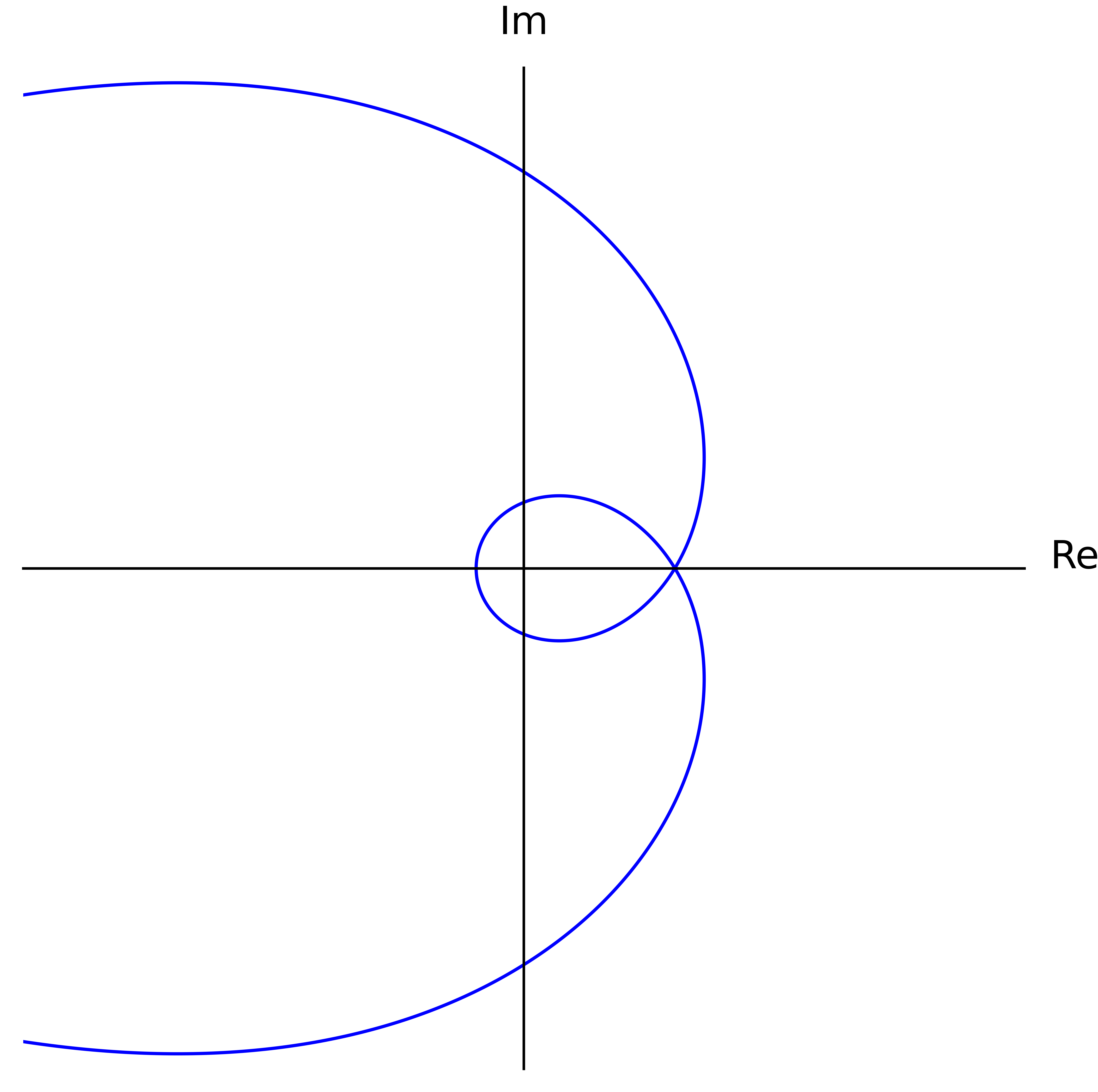
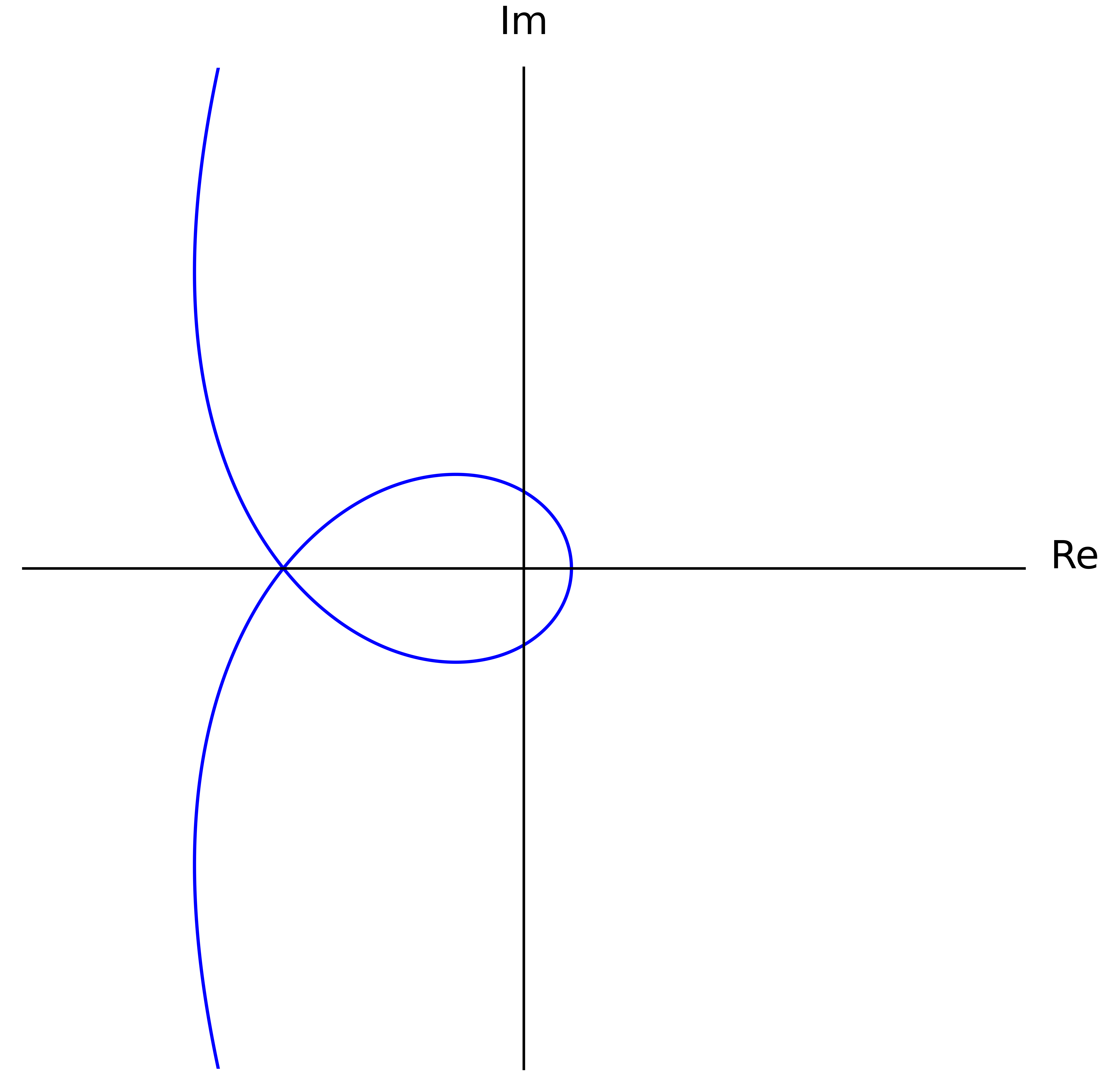
In our case for @@I_{-\infty}^\infty \frac{p_i(t)}{p_r(t)}@@, the poles considered by the Cauchy index correspond to the values of @@t@@ where @@\gamma@@ crosses the imaginary axis. In other words, it captures when @@\gamma@@ changes which side of the complex plane it's on — either the left or the right half. When we change sides, we can pass the origin either clockwise or counterclockwise. This "rotation information" is what's tracked by the Cauchy index, as shown in the figure above. Transitioning counterclockwise contributes @@-1@@ to the sum since @@\frac{p_i(t)}{p_r(t)}@@ goes from positive to negative at that value of @@t@@. Likewise, transitioning clockwise contributes @@+1@@. Now it turns out, this rotation information at each side-change is sufficient to compute the final winding number. In the end, each counterclockwise transition contributes @@+\frac{1}{2}@@, and each clockwise @@-\frac{1}{2}@@. For example, suppose @@\gamma@@ happens to come in from the left, then pass under the origin (counterclockwise). If no further transitions were to happen⁹, @@\gamma@@ would have to exit along the positive real axis, and the final winding number would be forced to be @@+\frac{1}{2}@@. If instead the path continued by passing above the origin (counterclockwise), then it would be forced to exit along the negative real axis assuming no further transitions, and the final winding number would be @@+\frac{2}{2}@@. Similarly if instead it then passed under the origin (clockwise), then again it would be forced to exit left, but this time with a final winding number of zero. Ultimately, we can get away with only looking at the side transitions since @@\gamma@@ can only enter and exit along the real axis.

To summarize, all counterclockwise passes contribute @@+\frac{1}{2}@@ to the winding number and @@-1@@ to the Cauchy index, while all clockwise passes count for @@-\frac{1}{2}@@ and @@+1@@ respectively. Taking care of the signs, we have

%% \begin{align*} \frac{1}{2\pi} \Delta \arg \left[ \gamma \right] = \frac{1}{2}(n_L-n_R) &= -\frac{1}{2} \cdot I_{-\infty}^\infty {\textstyle \frac{p_i(t)}{p_r(t)}} \nl n_L - n_R &= -I_{-\infty}^\infty {\textstyle \frac{p_i(t)}{p_r(t)}}. \end{align*} %%

This formula only works for even degree polynomials. For odd degree polynomials, the logic is the same, but we're looking at transitions between the top and bottom halves of the complex plane. Since these transitions happen where the imaginary part is zero, the end result is related to the Cauchy index of @@\frac{p_r(t)}{p_i(t)}@@ instead. In the end,

%% n_L - n_R = \begin{cases} -I_{-\infty}^\infty {\textstyle \frac{p_i(t)}{p_r(t)}} & \text{if $n$ is even} \nl +I_{-\infty}^\infty {\textstyle \frac{p_r(t)}{p_i(t)}} & \text{if $n$ is odd} \nl \end{cases}. %%

Eve's Theorem

With all the groundwork we've laid so far, the proof of Eve's theorem is mostly straightforward, though there is also a creative technique it uses to increase its strength. In short, Eve's theorem says that if almost all of the roots of some polynomial @@p@@ lie on one half of the complex plane — either the left or the right half, then all the roots of @@p_o@@ are real. The original proof uses the properties of Cauchy indices to prove this, but I find it more instructive to think of it in terms of the path @@\gamma(t) = p(it)@@.

First though, we can perform a few simplifications. Without loss of generality, let's assume most of the roots are on the left side, with real part at most zero. If that's not the case, we can instead run this argument on @@q(z) := p(-z)@@. This has the effect of swapping the sides of each of the roots. But note that

%% p(-z) = p_e(z^2) - z \cdot p_o(z^2), %%

so @@q_e(z) = p_e(z)@@ and @@q_o(z) = -p_o(z)@@. Since this argument shows that all the roots of @@q_o@@ are real, it follows that all the roots of @@p_o@@ are as well. Without loss of generality, we may also assume that no roots are on the imaginary axis. The Routh-Hurwitz theorem doesn't handle that case, but Eve's theorem does. If @@p(iy) = 0@@ for some @@y@@, then @@-y^2@@ is a common root of @@p_e@@ and @@p_o@@; remember how we decomposed @@p(it)@@ earlier. So, we can just factor that root out before proceeding with this argument.

"Weak" Version

For now, assume all @@n@@ roots of @@p@@ are in the left half of the complex plane. The full version of Eve's theorem weakens this requirement slightly, making it stronger overall, but a lot of the proof ideas carry over. Regardless, by the Routh-Hurwitz theorem, the winding number of @@\gamma@@ about the origin is @@+\frac{n}{2}@@. We're going to use that winding number to lower-bound how many real roots @@p_i@@ and thus @@p_o@@ have, ultimately showing all of @@p_o@@'s roots are real.

Consider the case where @@n@@ is even. In order to get the winding number as high as @@+\frac{n}{2}@@, @@\gamma@@ must cross the imaginary axis counterclockwise at least @@n@@ times, using the ideas from the previous section. And in fact, those crossings must be the only ones, since @@p_r@@ has at most @@n@@ real roots because of the bounds on its degree. Finally, since those crossings of the imaginary axis have to alternate above and below the origin (just look at the figure), @@\gamma@@ must cross the real axis at least @@n-1@@ times between them (by fencepost). This gives @@\Im[\gamma(t)] = p_i(t)@@ at least @@n-1@@ real roots. And this is also exact since the degree of @@p_i@@ for even @@n@@ is at most @@n-1@@.

Ignoring the extra root at zero, the roots of @@p_i@@ form @@\frac{1}{2}(n-2)@@ positive/negative root pairs, since @@\frac{1}{z} p_i(z)@@ is even.¹⁰ Hence, we can write

%% \begin{align*} p_i(z) &= z \cdot \prod_{a = 1}^{\frac{1}{2}(n-2)} (z + r_a)(z - r_a) \nl &= z \cdot \prod_{a = 1}^{\frac{1}{2}(n-2)} (z^2 - r_a^2) \nl &= z \cdot \prod_{a = 1}^{\frac{1}{2}(n-2)} -((-z^2) + r_a^2). \end{align*} %%

Pattern matching gives

%% p_o(z) = \prod_{a = 1}^{\frac{1}{2}(n-2)} -(z + r_a^2), %%

so @@p_o@@ has @@\frac{1}{2}(n-2)@@ real roots, at @@-r_a^2@@ for each @@a@@. Finally, since the degree of @@p_o@@ is at most @@\frac{1}{2}(n-2)@@ when @@n@@ is even, we conclude that all the roots of @@p_o@@ are real.

The case for @@n@@ odd is analogous and in some respects even easier. Here, @@p_i@@ has at exactly @@n@@ real roots due to the winding number forcing that many crossings of the real axis. Ignoring the extra root at zero, we get @@\frac{1}{2}(n-1)@@ root pairs. Those give rise to @@\frac{1}{2}(n-1)@@ real roots in @@p_o@@, which accounts for all of them.

In the presence of stronger assumptions on the roots than what the full version makes, we seem to actually have proven a statement stronger than what's given in the consequent of Eve's theorem. First, we seem to have shown that all the roots of @@p_o@@ are non-positive real numbers. Furthermore, our analysis of @@\gamma@@ additionally showed that the real roots of @@p_i@@ are all distinct, since @@\gamma@@ must physically cross the real axis @@n-1@@ times. Propagating this through seems to show that all the roots of @@p_o@@ are distinct too, since the root pair @@\pm r_a@@ only shows up once in @@p_i@@'s factorization.

Full Version

The actual formulation of Eve's theorem says something stronger: it also allows a single root to be in the right half of the complex plane, while the remaining @@n-1@@ roots stay in the left half. This makes @@\gamma@@'s winding number @@\frac{1}{2}(n-2)@@.

For even @@n@@, analyzing @@\gamma@@ the same way as in the last section, we only guarantee @@n-2@@ crossings and at least @@n-3@@ real roots for @@p_i@@ between them. Miraculously, this is still enough to show that all the roots of @@p_o@@ are real. To see this, observe that if @@p_i(r) = 0@@, then the same is true for @@r^*@@, @@-r@@, and @@-r^*@@. If @@p_i@@ had a complex root — one that's not on the real nor imaginary axes, then all four of these numbers would be distinct. Combining them with the @@n-3@@ real roots we already have, we'd get @@n+1@@ roots in total, which is impossible since @@p_i@@ has degree at most @@n@@. Therefore, all of @@p_i@@'s roots are either real or purely imaginary. That means the square of each of its roots is a real number, so we can repeat the process from the last section to get

%% p_o(z) = \prod_{a = 1}^{\frac{1}{2}(n-2)} -(z + r_a^2). %%

Here, each of @@p_o@@'s @@\frac{1}{2}(n-2)@@ roots @@-r_a^2@@ are real, though they're not necessarily non-positive.

When @@n@@ is odd, we similarly conclude @@p_i@@ has at least @@n-2@@ real roots, at which point the same argument in the last paragraph allows us to conclude that all the roots of @@p_o@@ are real.

Application to Knuth's Algorithm

Finally, we arrive at the algorithm that motivated this entire exploration. We'll consider a polynomial @@p : \RR \to \RR@@. We want to make an algorithm that evaluates @@p@@ at an arbitrary @@x \in \RR@@ using as few real-number operations as possible. Knuth's approach to this problem is to split

%% p(x) = p_e(x^2) + x \cdot p_o(x^2). %%

Now suppose @@p_o@@ has a real root @@r@@. Then we can factor it out of @@p_o@@, and we can divide it out of @@p_e@@ to get a real number as a remainder. In the end,

%% \begin{align*} p_o(x) &= (x - r) \cdot q_o(x) \nl p_e(x) &= (x - r) \cdot q_e(x) + c, \end{align*} %%

so

%% \begin{align*} p(x) &= (x^2 - r) \cdot q_e(x^2) + c + x \cdot (x^2 - r) \cdot q_o(x^2) \nl &= (x^2 - r) \cdot \left( q_e(x^2) + x \cdot q_o(x^2) \right) + c \nl &= (x^2 - r) \cdot q(x) + c. \end{align*} %%

We can apply this approach recursively to @@q@@ to get an algorithm for evaluating @@p(x)@@. And it's a great algorithm! Assuming we precompute @@x^2@@, each recursive step to reduce the degree of @@p@@ by two requires two additions and just one multiplication. In total, to evaluate a polynomial of degree @@n@@, we need @@n+O(1)@@ additions and @@\frac{1}{2}n+O(1)@@ multiplications, which is the best possible.

Sadly, running this algorithm to completion requires all the roots of @@p_o@@ to be real. We could try to allow @@r@@ to be complex. Unfortunately, then the algorithm starts requiring complex additions and multiplications, which are twice and four times as expensive as the corresponding real operations respectively, and the advantage of Knuth's algorithm fizzles out.

Luckily, we have Eve's theorem, which sometimes guarantees that all the roots of @@p_o@@ are real. Furthermore, given an arbitrary polynomial @@p@@, we can "preprocess" it to satisfy the premises of the theorem. Specifically, we can shift most of its roots to the left half of the complex plane by constructing @@q(x) := p(x + s)@@ for some sufficiently large @@s@@. We can then run Knuth's algorithm to evaluate @@q@@ at @@x - s@@, giving @@p(x)@@.

%% \begin{align*} p(x) &= x^n + c_{n-1} x^{n-1} + \cdots + c_1 x + c_0 \nl &= (x-r_1) \cdot \cdots \cdot (x-r_n). \end{align*} %%

Let's call this function @@\mathcal{V} : \CC^n \to \CC^n@@. Now, @@\mathcal{V}@@ is continuous — in fact it's holomorphic, as can be seen by just expanding the product and looking at the resulting coefficients. Furthermore, the inverse is "locally continuous". That's not the technical term; I invented it. What I mean is that if @@\mathcal{V}(\mathbf{r}) = \mathbf{c}@@, then for any small perturbation to @@\mathbf{c}@@ called @@\mathbf{c}^\prime@@, I can find a small perturbation to @@\mathbf{r}@@ called @@\mathbf{r}^\prime@@ such that @@\mathcal{V}(\mathbf{r}^\prime) = \mathbf{c}^\prime@@. I didn't prove this; I just intuited it by Taylor-expanding polynomial in question about each root.

Apparently, this map has a name; @@\mathcal{V}@@ is the Viète map. That name comes from this StackExchange thread. It mainly looks at showing the statement from the last paragraph — that the roots of a polynomial locally depend continuously on its coefficients. Turns out, it's not obvious how to prove that. My intuition works for square-free polynomials, and this Wikipedia page says that the holomorphic implicit function theorem gives the required result in that case. I also like the proof given by Alexandrian,¹ since it uses complex analysis rather than topology.

Regardless, I think another way to state my observation is: the set @@\CC^n@@ covers itself multiple times.² In fact, it @@n!@@-covers itself, since every permutation of the roots maps to the same sequence of coefficients. I'm not entirely sure why, but this was surprising to me. In the context of sets, there are things like Hilbert's Hotel and Banach–Tarski. The latter is more relevant here, since (one formulation of) it shows that @@S^2@@ can "map over" itself twice. Neither of these examples use continuous functions though, and I thought enforcing continuity would prevent this from happening. Obviously, not the case.

This isn't even the simplest example of multiple-covering I can think of. The circle @@S^1 \cong \RR / 2\pi\ZZ@@ covers itself any number of times. For any positive integer @@k@@, simply do @@t \mapsto k \cdot t@@. In a similar vein, the punctured complex plane @@\CC \setminus \{0\}@@ @@k@@-covers itself via the map @@z \mapsto z^k@@.

I started wondering if I could use @@\RR@@ to cover itself exactly @@k@@ times, for any positive number @@k@@. At first, I considered a weaker condition:³

Definition: I'll say that a continuous function @@f: X \to Y@@ @@k@@-hits @@Y@@ if, for every @@y@@, there are exactly @@k@@ distinct @@x@@ such that @@f(x) = y@@. If @@k \geq 2@@, then I'll say that @@f@@ multiple-hits @@Y@@.

I make this definition by analogy to covering. It drops the requirement that @@f@@ locally be a homeomorphism, meaning it also doesn't have to have a locally continuous inverse.

At first, I thought it was impossible to multiple-hit @@\mathbb{R}@@ from @@\mathbb{R}@@ itself. Polynomials have been on my mind recently, and indeed it is impossible for polynomials.

Observation: For any polynomial @@p : \RR \to \RR@@, there is some infinite interval @@I@@ containing points such that, for any @@y \in I@@, @@p(x) = y@@ has at most one solution.

First note that @@p@@ will eventually become monotonic as @@x \to \pm \infty@@. So let @@p@@ be monotonic on @@L := (-\infty, x_\min)@@ and on @@R := (x_\max, \infty)@@. The polynomial @@p@@ need not have the same "tonicity" on @@L@@ and @@R@@; it could be monotonically increasing on one and monotonically decreasing on the other. Regardless, the extreme value theorem gives that, on the interval @@M := [x_\min, x_\max]@@, @@p@@ attains a minimum and maximum @@y_\min@@ and @@y_\max@@ respectively.

Now consider two candidate intervals @@I_- = (-\infty, y_\min)@@ and @@I_+ = (y_\max, \infty)@@. By construction, no @@x \in M@@ can cause @@p@@ to evaluate to a @@y \in I_- \cup I_+@@, so any solutions there must come from @@L@@ or @@R@@. Using the monotonicity of @@p@@ and the fact that

%% y_\min \leq p(x_\min) = p(x_\max) < y_\max, %%

we see that in fact each of @@L@@ and @@R@@ contribute at most one solution to @@y@@s in either @@I_-@@ or @@I_+@@ (but not both). Doing casework, we can choose one of those intervals to be the returned result. □

This observation can be made even stronger: if some @@y \in I@@ has a solution, then all of them do. That can be shown by using the fact @@\lim_{x \to \pm \infty} p(x) = \pm \infty@@.

So polynomials are not enough. Still, the technique of "sign analysis", which I originally learned for polynomials,⁴ can sometimes be applied to continuous functions.

Definition: Let @@f@@ by a continuous function such that @@f(x) = y@@ has finitely many solutions @@x_1, \cdots, x_k@@. I define the sign chain of @@f@@ at @@y@@, which I denote @@\chn{f}{y}@@, as the list of length @@k+1@@ containing whether @@f@@ is greater than (@@+@@) or less than (@@-@@) @@y@@ on the subintervals @@(-\infty, x_1)@@, @@(x_1, x_2)@@, …, @@(x_k, \infty)@@.

So for example, consider the function @@x^3 - x@@. Its sign chain at @@y = 0@@ is @@[-, +, -, +]@@, while at @@y = 1@@ it's @@[-, +]@@. Note that the sign chain doesn't have to alternate. Consider @@\chn{x^2}{0} = [+, +]@@.

This notion is well-defined. No subinterval can contain an @@x@@ where @@f(x) = y@@. If one does, we missed a solution. Furthermore, no subinterval can contain @@x_a, x_b@@ such that @@f(x_a) < y@@ and @@f(x_b) > y@@ or vice versa. If one does, then the intermediate value theorem can find a solution we missed.

Definition: If @@c@@ is a sign chain, I define the sign of that sign chain, which I denote @@\sgn{c}@@, as even (@@+1@@) if consecutive elements of @@c@@ differ an even number of times, and odd (@@-1@@) otherwise. Equivalently, @@\sgn{c}@@ is even if the first and last elements of @@c@@ are the same, and odd if they are different.

So for example, @@\sgn{[-, +, -, +]} = -1@@, while @@\sgn{[+, +]} = +1@@.

Usually, we were interested in sign chains of polynomials at zero. Those are particularly helpful for plotting, and they have some nice properties. For example, the sign of any sign chain for any polynomial concides with the parity of that polynomial's degree, and the sign difference between consecutive elements of the sign chain at zero gives the parity of the multiplicity of the corresponding root.

Returning to our original goal of multiple-hitting @@\RR@@ though, we have the following.

Lemma: Let @@f : \RR \to \RR@@ be a surjective continuous function, and let @@f(x) = y@@ have only finitely many solutions @@x_1, \cdots, x_k@@ for some @@y@@. Then, @@\sgn{\chn{f}{y}} = -1@@.

We'll prove the contrapositive. Assume @@\sgn{\chn{f}{y}} = +1@@, and without loss of generality assume the first entry in @@\chn{f}{y}@@ is a @@+@@. Then the last entry is also a @@+@@ due to the sign of the sign chain. Ultimately @@f(x) > y@@ when @@x \in (-\infty, x_1) \cup (x_k, \infty)@@. Furthermore, the extreme value theorem bounds @@f(x) \in [y_\min, y_\max]@@ when @@x \in [x_1, x_k]@@. Note that, @@y \geq y_\min@@ since @@y = f(x_1)@@ and @@y = f(x_k)@@ by definition. No matter where @@x@@ is located, we have that @@f(x) \geq y_\min@@, so @@f@@ cannot be surjective. □

Theorem: If @@f : \RR \to \RR@@ @@k@@-hits, then @@k@@ is odd.

Start by picking any @@y@@. Let @@x_1, \cdots, x_k@@ be the solutions to @@f(x) = y@@, and let @@c = \chn{f}{y}@@. Now we'll consider offsetting @@y@@ by a small amount. For now, we'll consider shifting it up to @@y + \epsilon@@. If we do this, every subinterval @@(x_i, x_{i+1})@@ of @@c@@ where @@f(x) > y@@ — every "interior" @@+@@ subinterval — gives at least two solutions to @@f(x) = y + \epsilon@@. To see this, choose @@\epsilon@@ small enough that

%% f(x_i), f(x_{i+1}) = y < y + \epsilon < \max_{x \in (x_i, x_{i+1})} f(x). %%

⁵ The intermediate value theorem gives at least two crossing points: one on the way up to the maximum from @@f(x_i)@@, and one on the way back down from the maximum to @@f(x_{i+1})@@.

Now for the "exterior" subintervals. Due to the previous lemma, exactly one of those two subintervals of @@c@@ — either @@(-\infty, x_1)@@ or @@(x_k, \infty)@@ — is @@+@@ and thus has @@f(x) > y@@. Without loss of generality, let's say its the left one. This subinterval gives at least one solution to @@f(x) = y + \epsilon@@. Again, choose any @@\epsilon@@ small enough that

%% f(x_1) = y < y + \epsilon < \sup_{x \in (-\infty, x_1)} f(x). %%

⁶ If we do that, we have @@f(x) > y + \epsilon@@ for some @@x \in (-\infty, x_1)@@, at which point the intermediate value theorem gives a point with equality.

In the end, if @@n_+@@ is the number of @@+@@ intervals in @@c@@, then @@f(x) = y + \epsilon@@ has at least @@2n_+ - 1@@ solutions. The @@n_+ - 1@@ interior subintervals contribute at least two solutions each, and the one exterior subinterval gives at least one more. Now since @@f@@ @@k@@-hits @@\RR@@, we have

%% 2n_+ - 1 \leq k. %%

We considered shifting @@y@@ up by a small amount here, but we could've shifted it down by a small amount. Doing analogous steps gives

%% 2n_- - 1 \leq k. %%

And of course, every subinterval is either @@+@@ or @@-@@, so @@n_+ + n_- = k + 1@@, which is the length of the whole list @@c@@.

Now, algebra. We can sum the two inequalities to find that

%% 2n_+ + 2n_- \leq k + 2. %%

But doubling the equality constraint gives

%% 2n_+ + 2n_- = k + 2. %%

The only way for this to work is for both the inequalities to be tight. In other words,

%% \begin{align*} n_+,n_- &= \frac{k+1}{2}. \end{align*} %%

Since @@n_+@@ and @@n_-@@ are both integers, this only works if @@k@@ is odd. □

(I really hope this proof is correct. I don't fully understand how badly behaved continuous functions can be though!)

So that gives us some constraints on what multiple-hitting functions look like. But can we get a concrete example? I found this:

%% \mathcal{H}_1(x) = x + H_1 \cdot T(x), %%

where

%% T(x) = \begin{cases} \{x\} & \text{if } \{x\} \leq \frac{1}{2} \nl 1 - \{x\} & \text{if } \{x\} \geq \frac{1}{2} \end{cases}, %%

@@\{x\} = x - \lfloor x \rfloor@@ is the fractional part of the real number @@x@@, and @@H_1@@ happens to be @@3@@. The function @@T@@ is a triangle wave starting at zero with a period of one and spanning @@[0, \frac{1}{2}]@@. This function seems to @@3@@-hit @@\RR@@, as shown in the plot below. Sweeping up the @@y@@-axis, each "trough" creates a new solution which then splits into two. These two solutions go to the two adjacent "peaks", where they each merge with another solution, then annihilate. The scaling factor @@H_1@@ times it so that a solution pair is annihilated precisely when a new one is created, so overall the number of solutions always remains the same.

In general, it seems this framework can be used to create functions that @@(2t + 1)@@-hit @@\RR@@, for all positive integers @@t@@. Because of the theorem above, this framework gives examples of functions that @@k@@-hit @@\RR@@ for every possible value of @@k@@ (except for the trivial @@k = 1@@ case). We just set

%% H_t = 2t + 1. %%

I got that value by solving for when the trough at @@x = 0@@ is at the same height as the peak at @@x = -\frac{1}{2}(2t + 1)@@.

Even though these @@\mathcal{H}_t@@ functions multiple-hit @@\mathbb{R}@@, they don't multiple-cover @@\mathbb{R}@@ since their inverse isn't locally continuous. To see this, observe that at @@x = 0@@ the output is @@y = 0@@. But if nudge the output down slightly to @@y = -\epsilon@@, I can't make a small nudge to the input to acheive that output, since it's in the middle of a trough. I think this is fundamental:

Conjecture: No simply connected topological space admits a (non-trivial) multiple-covering.

This statement is actually true; see this StackExchange thread and this blog post. I just don't know the machinery to prove it, so I mark it as a conjecture.

If we require the covering space @@p : \tilde{X} \to X@@ to be path-connected, I think I want to do the following. Suppose @@x \in X@@ has two preimages @@\tilde{x}_0@@ and @@\tilde{x}_1@@. Let @@\tilde{\gamma}@@ be a path in @@\tilde{X}@@ between those two points. Under @@p@@, that path maps to a loop @@\gamma@@ in @@X@@. But since @@X@@ is simply connected, we can contract @@\gamma@@ to a point. I want to continuously deform @@\tilde{\gamma}@@ so that it always maps to @@\gamma@@ throughout the contraction.

In the end, @@\tilde{\gamma}@@ would be a path from @@\tilde{x}_0@@ to @@\tilde{x}_1@@, while @@\gamma@@ is constant at @@x@@. We'd get an entire continuous path of points mapping to the same point. And because @@p@@ is a covering, this would give a large family of open sets in @@\tilde{X}@@, each disjoint from each other, and each homeomorphic to a particular open set containing @@x@@. This is certainly weird. It should be possible to derive a contradiction from here, or at the very least to add more conditions to @@\tilde{X}@@ to cause a contradiction. □

At the very least, this conjecture is consistent with the datapoints we've collected so far. The circle @@S^1@@ and the nonzero complex numbers @@\CC \setminus \{0\}@@ both can be multiple-covered — by themselves in fact — and are both not simply connected. You may object, saying that the map that started this whole adventure @@\mathcal{V} : \CC^n \to \CC^n@@ is a counterexample. Unfortunately, I lied. The Viète map fails to be a covering space since, even though it is locally invertible, it is not uniquely locally invertible. If I have @@\mathcal{V}(\mathbf{c}) = \mathbf{r}@@, and I make a small adjustment to get @@\mathbf{r}^\prime@@, I may have multiple choices for @@\mathbf{c}^\prime@@. As an example, consider @@\mathbf{r} = x^2@@ and @@\mathbf{c} = (x-0)\cdot(x-0)@@. If I perturb @@\mathbf{r}^\prime = x^2 - \epsilon^2@@, then I can choose between @@\mathbf{c}^\prime = (x + \epsilon) \cdot (x - \epsilon)@@ or @@(x - \epsilon) \cdot (x + \epsilon)@@. Order matters here since we're viewing these as vectors.

We can restrict @@\mathcal{V}@@ by forcing its inputs to have distinct elements. In that case, it would map from the configuration space @@\Conf{\CC}{n}@@ to some subset of @@\CC^n@@. It wouldn't map to the whole space though, so it wouldn't constitute a multiple-cover. Still,

Theorem: Assuming @@n \geq 2@@, @@\Conf{\CC}{n}@@ is not simply connected.

Intuitively, we're starting with something that looks like a real vector space of dimension @@2n@@ and removing a finite number of subspaces of dimension @@2n - 2@@. This space is path connected because disconnecting @@\RR^{2n}@@ requires removing a subspace of dimension @@2n-1@@ or higher. It's not simply connected since we can create non-contractible loops by wrapping a path, occupying a two-dimensional plane, around one of the subspaces we removed.

Formally, I'll just show that there exist non-contractible loops in @@\Conf{\CC}{n}@@.⁷ Suppose for the sake of contradiction that the path

%% \gamma(t) = \begin{pmatrix} e^{2\pi i \cdot t} & -e^{2\pi i \cdot t} & z_3 & \cdots & z_n \end{pmatrix}^\intercal %%

is contractible to a point. It doesn't matter what the higher components @@z_3, \cdots, z_n@@ are exactly, as long as they are distinct and don't lie on the unit circle. Now look at the function

%% f(\mathbf{z}) = z_1 - z_2 %%

that subtracts the first two components of the supplied vector. If the domain of @@f@@ is taken to be @@\Conf{\CC}{n}@@, then the range of @@f@@ is the punctured complex plane @@\CC \setminus \{0\}@@ because @@z_1 \neq z_2@@.

Now, @@f \circ \gamma@@ is a continuous loop in that plane. In fact, it is the loop that starts at @@2@@ and encircles the origin once counterclockwise. But if @@\gamma@@ is contractible to a point, then @@f \circ \gamma@@ is as well — indeed, a small adjustment to the input loop gives a small change to the output loop. But it's known that continuously contracting a loop encircling the origin down to a point is impossible. □

Corollary: The image @@\mathcal{V}(\Conf{\CC}{n})@@ is not simply connected.

From above, consider @@\mathcal{V} \circ \gamma@@. By assumption, the resulting loop is contractible to a point, so all of the preimages of that loop can also be contracted; this comes from the homotopy lifting property. But the argument above shows that can't happen in this case. □

I think I'm gonna end things off here. This was an interesting rabbit hole to dive down. I've never had any formal training in topology or even analysis; I studied to be a computer scientist, after all. Still, I think I learned a good deal by trying to understand statements made in the languages of those areas. Either way, I think I'd have an easier time picking them up if I have to in the future.

The strategy I came up with was to factor the polynomial in question @@p@@ into quadratics, writing¹

%% p(x) = k \cdot (x^2 + a_1 x + b_1) \cdots (x^2 + a_{N/2} x + b_{N/2}). %%

This is always possible due to the fundamental theorem of algebra and the complex conjugate root theorem. We write @@p@@ this way because it naturally gives a parallel algorithm for evaluating @@p(x)@@. Each factor is evaluated in parallel, then a reduction network is used to multiply them all together.

With this Factorization-Based Algorithm, each of the @@N/2@@ terms needs two adders, but just one multiplier since the @@x^2@@ can be computed once and reused across all the terms. The final reduction needs @@(N/2 + 1) - 1 = N/2@@ multipliers. In total, @@N@@ adders and @@N@@ multipliers are needed. So, this algorithm matches the hardware requirements of Horner's Scheme. However, its critical path is much shorter. Each factor has one multiplier and two adders on its critical path, and the final reduction has a critical path of @@\lceil \log(N/2+1) \rceil@@² multipliers. Compare these figures to Estrin's Scheme, which has @@\lceil \log(N+1) \rceil@@ multipliers and @@\lceil \log(N+1) \rceil@@ adders on its critical path. Ultimately, preprocessing allows this Factorization-Based Algorithm to achieve a shorter critical path than Estrin's Scheme while also saving area.

Claude suggested that I add worked example for this algorithm. So, consider @@N=5@@ and

%% p(x) = x^5 + 2x^4 + 3x^3 + 4x^2 + 5x + 6. %%

The polynomial @@p@@ has roots

%% \begin{align*} r_1 &\approx -1.492 \nl r_2 &\approx -0.806 + 1.223i \nl r_3 &\approx -0.806 - 1.223i \nl r_4 &\approx 0.552 + 1.253i \nl r_5 &\approx 0.552 - 1.253i. \end{align*} %%

The roots @@r_2@@ and @@r_3@@ are conjugates, as are @@r_4@@ and @@r_5@@. Those roots have to be merged to form quadratics, while the remaining roots can be merged. Ultimately, we write

%% p(x) = k \cdot (x + b_0) \cdot (x^2 + a_1 x + b_1) \cdot (x^2 + a_2 x + b_2), %%

where the constants are chosen such that

%% \begin{align*} k &= 1 \nl x + b_0 &= (x - r_1) \nl x^2 + a_1 x + b_1 &= (x - r_2) \cdot (x - r_3) \nl x^2 + a_2 x + b_2 &= (x - r_4) \cdot (x - r_5). \end{align*} %%

This particular case gives

%% \begin{align*} b_0 &\approx 1.492 \nl a_1 &\approx 1.612 \nl b_1 &\approx 2.145 \nl a_2 &\approx 1.103 \nl b_2 &\approx 1.875. \end{align*} %%

All of the work above only has to be done once, offline. The hardware will only see these coefficients, at which point it can run the data-flow graph given below.

flowchart TB
  xsqin[$$x$$]
  xsq[$$x^2$$]
  sq[$$\times$$]
  xsqin --> sq
  xsqin --> sq
  sq --> xsq

  x0[$$x$$]
  b0[$$b_0$$]
  add0[$$+$$]
  x0 --> add0
  b0 --> add0

  xsq1[$$x^2$$]
  x1[$$x$$]
  a1[$$a_1$$]
  b1[$$b_1$$]
  mult1[$$\times$$]
  add1lo[$$+$$]
  add1hi[$$+$$]
  a1 --> mult1
  x1 --> mult1
  mult1 --> add1lo
  b1 --> add1lo
  xsq1 --> add1hi
  add1lo --> add1hi

  xsq2[$$x^2$$]
  x2[$$x$$]
  a2[$$a_2$$]
  b2[$$b_2$$]
  mult2[$$\times$$]
  add2lo[$$+$$]
  add2hi[$$+$$]
  a2 --> mult2
  x2 --> mult2
  mult2 --> add2lo
  b2 --> add2lo
  xsq2 --> add2hi
  add2lo --> add2hi

  red1[$$\times$$]
  red2[$$\times$$]
  add1hi --> red1
  add2hi --> red1
  add0 --> red2
  red1 --> red2

  red2 --> Output

That's all I have. It's not particularly original, but the idea of breaking a polynomial into factors does give rise to a pleasingly parallel algorithm. And note that the factoring doesn't have to continue all the way down to quadratics. It may be profitable to stop at some higher degree, especially since more efficient serial algorithms exist and it may not be possible to exploit such a high degree of parallelism. As a concrete example, perhaps when evaluating a polynomial of degree @@N=128@@, you could stop at factoring @@N=16@@ and use Knuth's Algorithm for those eight degree sixteen terms. Knuth's Algorithm would only require nine multipliers instead of the usual sixteen, but it is serial which makes the critical path longer. In other words, less area can be traded for greater latency. Also, this same idea — of breaking polynomials down recursively then using an efficient serial algorithm to evaluate them — is present in the Rabin-Winograd Algorithm

Another note: this Factorization-Based Algorithm heavily uses multipliers. They dominate the critical path, and either way more of them are used than in Knuth's Algorithm. This is by design. During my time on MINOTAUR, I observed that BFloat16 multipliers on our technology³ took half the time and less area than BFloat16 adders. Hence, this algorithm tries to keep adders off the critical path. If the balance were to shift in favor of addition, perhaps the naïve scheme would work better.

Finally, Claude suggested I consider numerical stability. It is known that small errors in roots can cascade into large errors in the final value. Considering we're using BFloat16 with just seven mantissa bits, and I intend to store all the coefficients with the same precision, the accuracy of the underlying model could tank. For what it's worth, no accuracy penalty was observed on MINOTAUR when using Horner's or Estrin's Schemes, or indeed when switching to piecewise cubic activations. But it's still possible this aggressive factorization causes too much error. But I haven't tested that, and frankly I don't think I will now that I'm off MINOTAUR.

I was not the only one working on the vector unit though. Another group looked at changing the strategy it used to compute activation functions. Ultimately, they settled on piecewise-cubic activations, with programmable coefficients and interval bounds. I interacted with them, and I investigated ways to make the computation of these cubic polynomials more efficient.

Let's say we have some

%% p(x) = c_3 x^3 + c_2 x^2 + c_1 x + c_0. %%

Naïvely implementing this in hardware, by evaluating all the multiplications before computing the additions, gives a relatively poor result. It requires six multipliers and three adders, and its critical path consists of two multipliers and two adders.

flowchart TB
    x3[$$x$$]
    x2[$$x$$]
    x1[$$x$$]

    c0[$$c_0$$]
    c1[$$c_1$$]
    c2[$$c_2$$]
    c3[$$c_3$$]

    c3m0[$$\times$$]
    c3m1[$$\times$$]
    c3m2[$$\times$$]
    c3 --> c3m0
    x3 --> c3m0
    x3 --> c3m1
    x3 --> c3m1
    c3m0 --> c3m2
    c3m1 --> c3m2

    c2m0[$$\times$$]
    c2m1[$$\times$$]
    c2 --> c2m0
    x2 --> c2m0
    c2m0 --> c2m1
    x2 --> c2m1

    c1m0[$$\times$$]
    c1 --> c1m0
    x1 --> c1m0

    a0[$$+$$]
    a1[$$+$$]
    a2[$$+$$]
    c3m2 --> a0
    c2m1 --> a0
    c1m0 --> a1
    c0 --> a1
    a0 --> a2
    a1 --> a2

    a2 --> Output

A better idea is to use Horner's Scheme, which decomposes @@p@@ as

%% p(x) = ((c_3 \cdot x + c_2) \cdot x + c_1) \cdot x + c_0. %%

It has a longer critical path, at three multipliers and three adders. But, it uses less area — just the three multipliers and three adders. Possibly for that reason, this was the initial scheme used in MINOTAUR. Area is particularly important for its vector unit. Most of its operations are performed on 32-wide vectors, pipelined and in parallel. So, any area savings are multiplied by 32.

flowchart TB
    x3[$$x$$]
    x2[$$x$$]
    x1[$$x$$]

    c0[$$c_0$$]
    c1[$$c_1$$]
    c2[$$c_2$$]
    c3[$$c_3$$]

    c3m[$$\times$$]
    c2a[$$+$$]
    c3 --> c3m
    x3 --> c3m
    c3m --> c2a
    c2 --> c2a

    c2m[$$\times$$]
    c1a[$$+$$]
    c2a --> c2m
    x2 --> c2m
    c2m --> c1a
    c1 --> c1a

    c1m[$$\times$$]
    c0a[$$+$$]
    c1a --> c1m
    x1 --> c1m
    c1m --> c0a
    c0 --> c0a

    c0a --> Output

Another improvement over the naïve approach is to use Estrin's Scheme, which instead recursively factorizes @@p@@ as

%% p(x) = x^2 \cdot (c_3 x + c_2) + (c_1 x + c_0). %%

In total, Estrin's Scheme uses four multipliers and three adders. Its critical path consists of two multipliers and two adders. In other words, for just an additional multiplier compared to Horner's Scheme, this algorithm improves on its critical path by a full Multiply-Accumulate (MAC). And in fact, when this approach was implemented in MINOTAUR, it saved area over Horner's Scheme. Its shorter critical path allowed the pipeline depth to be reduced by one stage, eliminating an entire set of pipeline registers.

flowchart TB
    xsq[$$x$$]
    xl[$$x$$]
    xr[$$x$$]

    c0[$$c_0$$]
    c1[$$c_1$$]
    c2[$$c_2$$]
    c3[$$c_3$$]

    sq[$$\times$$]
    xsq --> sq
    xsq --> sq

    ml[$$\times$$]
    al[$$+$$]
    c3 --> ml
    xl --> ml
    ml --> al
    c2 --> al

    mr[$$\times$$]
    ar[$$+$$]
    c1 --> mr
    xr --> mr
    mr --> ar
    c0 --> ar

    mt[$$\times$$]
    at[$$+$$]
    sq --> mt
    al --> mt
    mt --> at
    ar --> at

    at --> Output

The above approaches were actually synthesized in MINOTAUR. It's possible that they leave performance on the table though. Specifically, note that all the algorithms given above take the "raw" coefficients @@c_3@@, …, @@c_0@@ as input. But, Wikipedia's page on Polynomial Evaluation points out that pre-processing these coefficients can decrease the number of multipliers and adders required. Knuth's Algorithm¹ provides a concrete way to do that.

Knuth's Algorithm points out that, by applying polynomial long-division, we can write

%% p(x) = (x^2 + \alpha) (k_1 x + k_0) + \beta x + \gamma, %%

for some set of constants. The only knob we have is @@\alpha@@; once it's fixed, the divisor @@x^2 + \alpha@@ is set and the rest of the constants can be determined. The key idea is to judiciously set @@\alpha := \alpha^*@@ such that @@\beta = 0@@. This can be done by picking

%% \begin{align*} \alpha^* &= \frac{c_1}{k_1^*} \nl \gamma^* &= c_0 - \alpha^* k_0^* \nl k_1^* &= c_3 \nl k_0^* &= c_2, \end{align*} %%

which works so long as @@c_3 \neq 0@@. That case can be worked around for MINOTAUR. A few multiplexers can be used to reconfigure the existing multipliers and adders for Knuth's Algorithm to implement Horner's Scheme on quadratics. In the end, Knuth's Algorithm prescribes

def preprocess(c: list[float]):
    cubic = c[3] != 0
    if cubic:
        k1 = c[3]
        k0 = c[2]
        α = c[1] / k1
        ɣ = c[0] - α * k0
    else:
        k1 = c[2]
        k0 = c[1]
        α = float('nan') # Don't care
        ɣ = c[0]
    return (cubic, k1, k0, α, ɣ)

def hardware(
    x: float,
    cubic: bool,
    k1: float, k0: float, α: float, ɣ: float,
) -> float:
    quotient = k1 * x + k0
    divisor = x * x + α
    whole = quotient * divisor if cubic else quotient
    return whole + ɣ

def evaluate(x: float, c: list[float]) -> float:
    return hardware(x, *preprocess(c))

Ignoring MUX overhead, it requires three multipliers and three adders, and it has a critical path of two multipliers and two adders. Thus, it is strictly better than both Horner's and Estrin's Schemes. It does require preprocessing, but that's okay for MINOTAUR.

flowchart TB
    xq[$$x$$]
    xd[$$x$$]

    alpha[$$\alpha$$]
    gamma[$$\gamma$$]
    k0[$$k_0$$]
    k1[$$k_1$$]

    mq[$$\times$$]
    aq[$$+$$]
    k1 --> mq
    xq --> mq
    mq --> aq
    k0 --> aq

    md[$$\times$$]
    ad[$$+$$]
    xd --> md
    xd --> md
    md --> ad
    alpha --> ad

    mt[$$\times$$]
    at[$$+$$]
    aq --> mt
    ad --> mt
    mt --> at
    gamma --> at

    at --> Output

To close, even though none of the algorithms described here are entirely new, they don't seem to be widely known. For instance, I independently rediscovered Estrin's Scheme, and I came to Knuth's Algorithm myself after seeing a different algorithm inspired by it in a source I have since lost. Furthermore in my experience with MINOTAUR, Horner's Scheme is often treated as the "default" approach for polynomial evaluation in hardware, even when other approaches might be better. Either way, it was some work to find these algorithms, so hopefully this post can save someone else from doing redoing it.

Another question that remains is whether Knuth's Algorithm is "optimal". According to CS 497² at UIUC, it is known that Knuth's Algorithm uses the lowest possible number of multiplications and additions (or subtractions). But, it does not show that it achieves the best possible critical path. As shown by Estrin's Scheme in MINOTAUR, it may be better to optimize that instead of total area.

sameold

Hack ___ planet!

Submit a string that complies with the following rules:

• The string should start with the punycode of your team name. This is a good time for you to figure out with which team you are playing.
• After your team name, you may add any number of alphanumeric characters.
• CRC32(the_intended_answer) == CRC32(your_string)

Most teams solved this challenge by brute-force, which is surprisingly the intended solution. I can guess that this method "randomly" samples the possible checksums, taking @@2^{32}@@ tries to find a solution on average. This hunch is confirmed by all the example answers having six extra characters, where @@n=6@@ is the smallest integer satisfying @@62^n \geq 2^{32}@@. Finding a solution using fewer letters is possible but unlikely — @@21.7\%@@ probability at most.

However, there is another approach that leverages the properties of a Cyclic Redundancy Check (CRC). It is guaranteed to find a solution, and it does so much faster than the straightforward but exponential method.

Introduction

How CRCs Work

First, it's necessary to understand some of the math underlying CRCs. Ultimately, the goal of any checksum is to take in some data and derive from it a "check value" of a fixed length — 32-bit in our case. They just have to withstand random mutations, not adversarial changes to the input. As such, these algorithms can (and should) be simpler than hashes. They should be mathematically nice to ease reasoning about how they respond to different classes of errors and how those responses may be used to recover the original data from the corrupted copy.

In the specific case of CRCs, they treat each bit as an element of @@\FF_2@@: an element of @@\{0,1\}@@ where addition is XOR and multiplication is AND. This definition was chosen to make @@\FF_2@@ a field, a set where the usual operations (addition, subtraction, multiplication, division) are defined and behave the way you'd expect with regular numbers. To represent bitstrings, CRCs work over @@\FF_2[x]@@: the ring of polynomials with coefficients in @@\FF_2@@, with polynomial addition and multiplication defined in the usual way. For example, the string 1010 is represented as the polynomial @@x^3 + x@@, where @@x@@ is just a formal symbol not representing any underlying value. Again, this choice was made to make CRCs easy to reason about mathematically. Polynomials are some of the nicest objects out there, but they have just enough depth to admit sophisticated algorithms.

To calculate the checksum, CRCs reduce the bitstream's polynomial with respect to some modulus. For CRC-32, the modulus is %%\begin{align*} \pi =&\, 1 + x + x^2 + x^4 + x^5 \nl &+ x^7 + x^8 + x^{10} + x^{11} \nl &+ x^{12} + x^{16} + x^{22} + x^{23} \nl &+ x^{26} + x^{32}, \end{align*}%% the symbol @@\pi@@ of course standing for πolynomial. You can construct the message's polynomial and then take the remainder by polynomial long division, but it's more economical to do the reduction after each operation. Effectively, you work over @@\FF_2[x] / \langle\pi\rangle@@: the space of polynomials but you treat those that differ by some multiple of @@\pi@@ as equal. Again, long division can take any element to its "canonical" form.

That's CRCs in a nutshell. Treat your data as a polynomial @@p \in \FF_2[x] / \langle\pi\rangle@@ and reduce it to its canonical form by polynomial long division. Implementation is a bit more complicated than that, of course. For instance, you actually reduce @@p \cdot x^{32}@@. That way, you can just append the checksum to the message when sending it, and the check passes if the recieved data is congruent to zero modulo @@\pi@@. Additionally, some implementations perform superficial changes to the data. Some NOT the output. Some reflect the output's bits (so bit 31 maps to bit 0, 30 to 1, …). Some reflect the bits of each individual input byte.

Most importantly, many implementations use a table-driven approach, computing one byte at a time instead of just one bit. Exploring that is worth an entire post, but the upshot is that it's only equivalent to this method when the algorithm is seeded with zero. Some implementations seed it with 0xffffffff instead, which has the effect of NOTing the first 32 bits of the input. Equivalently, it prepends %%\begin{equation*} \frac{1}{x^{32}} \cdot \left( \sum_{i=0}^{31} x^i \right) \end{equation*}%% to the message. In general, if the table method is seeded with @@p@@, it XORs that with the first 32 bits of the input, or it equivalently prepends @@p \cdot x^{-32}@@.

The Choice of π

It's worth noting some properties of CRC-32's choice of @@\pi@@. That polynomial is irreducible over @@\FF_2@@, meaning it can't be factored any further without introducing numbers other than @@\{0,1\}@@. A nice result of this choice is that @@\FF_{2^{32}} = \FF_2[x] / \langle\pi\rangle@@ is itself a field. Every element has a multiplicative inverse, and it makes sense to talk about things like @@x^{-32}@@. The polynomial @@\pi@@ is also primitive, meaning the formal symbol @@x@@ generates the multiplicative group. Taking the powers of @@x@@ will go over every other element (except zero) before cycling back to @@x@@. Again, these choices were made to make reasoning about this structure easier.

The notation @@\FF_{2^{32}}@@ is no accident either. It's a field with exactly that many elements — a binary choice for each coefficient from @@x^0@@ to @@x^{31}@@. It's also the field with that many elements, since all of them are isomorphic. Additionally, all finite fields have prime power sizes, and it's worth exploring why that is, since the same methods are used in the attack later.

Lemma: A field @@F@@ can be viewed as a vector space over any of its subfields @@K@@.

The required axioms can easily be checked. Those for vector addition are almost trivially satisfied, as are those for identity and distributivity. The only important thing to check happens with vector multiplication. We require that %%\begin{equation*} a \cdot b\vect{v} = (ab) \cdot \vect{v} \end{equation*}%% where @@a,b \in K@@ and @@ab \in K@@. That's why we needed @@K@@ to be a subfield. □

An easy example is @@\FF_{2^{32}}@@ itself. The elements @@1, x, x^2, \cdots@@ can be thought of as basis "vectors," scaled by either zero or one: an element of @@\FF_2@@. This line of thinking extends quite well.

Theorem (from MathOverflow): A finite field @@F@@ has order @@|F| = p^n@@ for @@p@@ prime.

Consider the additive group generated by @@1@@, so %%\begin{align*} & 0 \nl & 0 + 1 \nl & 0 + 1 + 1 \nl & \cdots. \end{align*}%% It can be checked that these elements form a subfield @@K \subseteq F@@. Additionally, since @@F@@ is finite, continuting to add ones in this manner will eventually start to repeat elements, meaning @@K \cong \ZZ/p\ZZ@@. For that to be a field, @@p@@ must be prime.

By the lemma above @@F@@ is a vector space over @@K@@, and since it's finite, it's finitely generated. Let @@\{b_1, \cdots, b_n\}@@ be a basis, so every linear combination %%\begin{equation*} \alpha_1 b_1 + \cdots + \alpha_n b_n \end{equation*}%% gives a unique element of @@F@@. With each @@\alpha@@ in @@K@@, we get @@p@@ possibilities for each coefficient, giving a total of @@p^n@@ different elements. □

This is not the only proof of this theorem. Another, also from MathOverflow, uses Bézout's identity to show by contradiction that the field would have zero divisors otherwise.

Approach

With all the introductory material out of the way, we can start tackling the actual problem. As a reminder, we want to find a string that starts with a specific substring (say DC) whose CRC-32 is a particular value. I'll actually restrict the search space a bit more. I'll look for a string that starts with DC then contains exactly @@\ell@@ characters, each either @@c@@ or @@d@@. Let @@\delta = d - c@@ and compute @@p@@ the CRC-32 of the original message: DC followed by the character @@c@@ repeated @@\ell@@ times. Of course, this will likely differ from the target polynomial @@t@@, but we can change the message by substituting some instances of @@c@@ with @@d@@ — by adding instances of @@\delta@@ shifted by the appropriate amount. Intuitively, changing the message leads to predictable effects on the output — if you add something to the input, you just add the same thing to the output. So, we look at the difference and solve for the required change.

Specifically, we wish to solve for @@\alpha_i \in \FF_2@@ in %%\begin{equation*} x^{32} \cdot \sum_{i=0}^{\ell-1} \alpha_i \cdot x^{8i}\delta = t - p. \end{equation*}%% The @@x^{8i}@@ term in the sum shifts the correction into the right place. For example, setting @@i=0@@ will shift the correction to the last character in the string, setting @@i=1@@ will be the second to last, and so on. Choosing @@\alpha_i=1@@ means to substitute that character into @@d@@, while choosing it zero means to leave it as @@c@@. The extra shift of @@x^{32}@@ corresponds to the CRC algorithm multiplying the message by that before taking the remainder.

We can rearrange the above equation to read %%\begin{equation*} \sum_{i=0}^{\ell-1} \alpha_i \cdot \left(x^8\right)^i = \frac{t - p}{x^{32}\delta}. \end{equation*}%% On the LHS we have a linear combination of constant elements, and on the RHS we have a constant. To solve this, we suddenly remember that this field @@\FF_{2^{32}}@@ can be expressed as a vector space over a subfield. Taking @@K=\{0,1\}=\FF_2@@ allows us to operate under the standard basis @@\{1,x,x^2,\cdots,x^{31}\}@@. The constants can be rewritten in this basis to get %%\begin{align*} \sum_{i=0}^{\ell-1} \alpha_i \vect{v}_i &= \vect{y} \nl \matr{V}\vect{\alpha} &= \vect{y}, \end{align*}%% where @@\matr{V}@@ is the matrix with column vectors @@\vect{v}_i = x^{8i}@@. This system can be easily solved, though not necessarily uniquely, as long as @@\matr{V}@@'s columns span @@\FF_{2^{32}}@@.

Failure Resistance

So when does that fail? Clearly, when @@\ell@@ is too small, there aren't enough vectors for a baisis and thus too few for a spanning set. The least you can possibly get away with is @@\ell = \dim\FF_{2^{32}} = 32@@. In some cases, that's also sufficient.

On "2^w-Periodic" Bases

Specifically, when the attacker can choose to substitute individual words independently of each other, assuming a word's length is a power of two @@2^w@@, @@\ell=32@@ is sufficient. This is because going through the above process with this setup results in the vectors @@\vect{v}_i@@ being @@x^{2^w i}@@. I'll prove that this set is a basis iff the set of @@x^i@@ is a basis, which it obviously is for @@i = 0, \cdots, 31@@.

Theorem: The set @@B = \{b_0,\cdots,b_{\ell-1}\}@@ of elements in @@\FF_{p^n}@@ spans its field iff the set @@B^p = \{b_0^p,\cdots,b_{\ell-1}^p\}@@ does.

For the "only if" direction, observe that if @@v@@ can be expressed as a linear combination of basis elements in @@B@@, then %%\begin{align*} v^p &= \left( \sum_{i=0}^{\ell-1} \alpha_i b_i \right)^p \nl &= \sum_{i=0}^{\ell-1} \alpha_i^p b_i^p \nl \end{align*}%% by Freshman's Dream. Since the Frobenius endomorphism is bijective over finite fields, one can make any target vector out of elements of @@B^p@@ by making its preimage using @@B@@ then raising it to the @@p@@-th power.

For the "if" direction, we use a similar argument. To construct a target element @@v@@, construct @@v^p@@ using elements of @@B^p@@, then construct @@v@@ by taking the @@p@@-th root of all the coefficients and using them on the basis @@B@@. Again, doing this is well defined since the Frobenius endomorphism is bijective over @@\FF_{p^n}@@. □

Corollary: Same as the above theorem, but with the set @@B^{p^k} = \{b_0^{p^k},\cdots,b_{\ell-1}^{p^k}\}@@ instead of @@B^p@@, where @@k@@ is an arbitrary natural number.

Apply the above theorem @@k@@ times. □

The result we set out to prove is this corollary with @@p=2@@, @@k=w@@, and @@b_i = x^i@@.

On n Consecutive Powers of Primitive Elements

The result in the previous section was agnostic to our choice of @@b_i@@. However, our basis is usually quite "nice". For example, in the last section, we chose the standard basis @@\{1,x,x^2,\cdots,x^{31}\}@@. Moreover, since multiplication by a constant is a linear automorphism, we could have chosen any 32 consecutive powers of @@x@@. These same results hold for some other elements too.

In particular, it holds for primitive elements of @@\FF_{2^{32}}@@. This fact could've been used to prove the result in the last section. Unfortunately, it has limited utility since it requires consecutive powers of that element, which might be hard to guarantee for non-powers of two.

Lemma: If the minimal polynomial of @@g \in \FF_{p^n}@@ has degree at least (so, exactly) @@n@@, then the set @@\{1,g,g^2,\cdots,g^{n-1}\}@@ is linearly independent and therefore a basis for @@\FF_{p^n}@@.

I'll prove by contraposition. Suppose there were some constants @@\alpha_i \in \FF_p@@, not all zero, such that %%\begin{equation*} \sum_{i=0}^{n-1} \alpha_i g^i = 0. \end{equation*}%% Then by definition @@g@@ satisfies this polynomial nonzero of degree at most @@n-1@@, and its minimal polynomial must have degree less than or equal to that. □

Theorem: If @@g \in \FF_{p^n}@@ is primitive, then its minimal polynomial has degree at least (exactly) @@n@@.

Again, I'll proceed by contraposition. Without loss of generality, suppose @@g@@ satisfies some monic polynomial of degree @@d < n@@. We can move all the lower degree terms to one side to get %%\begin{equation*} g^d = \sum_{i=0}^{d-1} \alpha_i g^i. \end{equation*}%% Then, all subsequent powers of @@g@@ can be expressed as a linear combination of @@\{1,g,g^2,\cdots,g^{d-1}\}@@. Just keep substituting this identity until all instances of @@g@@ have power at most @@d-1@@. Therefore, the set of elements @@\langle g\rangle \subseteq \FF_{p^n}^\times@@ that can be reached via powers of @@g@@ has at most @@p^d - 1@@ elements. We get @@p@@ choices for each coefficient, minus one because zero can't be reached. This is strictly fewer elements than are contained in the whole field, so @@g@@ cannot be primitive. □

Corollary: If @@g \in \FF_{p^n}@@ is primitive, any @@n@@ consecutive powers of @@g@@ are linearly independent and therefore form a basis.

To show @@\{1,g,g^2,\cdots,g^n\}@@ is linearly independent, simply compose the above theorem and the lemma before it. As for any @@n@@ consecutive powers, with @@g^d@@ being the lowest power among them, linearly transform this basis via multiplication with @@g^d@@. □

Future Work

Characterizing powers of two and consecutive powers is relatively easy. However, real-world situations might not afford this structure. Attackers might only be able to choose bits at irregular positions, and the above guarantees about how many choices are needed to span might not hold. Future work might focus on getting a tighter bound on which and how many elements are needed to guarantee a spanning set.

Additionally, I assumed for simplicity that the attacker would choose once per byte — either @@c@@ or @@d@@. They usually have more choices than that though, and it would be good to take advantage of them. By introducing @@K@@ independent displacement vectors @@\delta_k@@, it's possible to use an alphabet @@\Sigma@@ that has @@2^K@@ characters. In that case, you need to solve %%\begin{align*} x^{32} \cdot \sum_{i=0}^{\ell-1}\sum_{k=1}^K \alpha_{i,k} \cdot x^{8i} \delta_k &= t - p \nl \sum_{i=0}^{\ell-1}\sum_{k=1}^K \alpha_{i,k} \cdot x^{8i} \delta_k &= \frac{t - p}{x^{32}}. \end{align*}%% Additionally, @@\Sigma@@ has to be an affine space over @@\FF_2@@, otherwise it wouldn't be possible to safely take linear combinations of the vectors @@\delta_k@@ as we require. Finally, while the bound on @@\ell@@ established above still technically holds, in the case of multiple displacement vectors, it's clearly very loose. Intuitively, we'd expect it to be close to @@\frac{32}{K}@@. Future work could try to relax these restrictions and get a tighter bound on the number of bytes needed.

Worked Example

Suppose I want to find a string that starts with DC, only contains the letters G and T after that, and whose CRC-32 is the same as the string the. I compute the target CRC to be 0x3c456de6, and undoing the post-processing by reversing the bits and NOTing gives %%\begin{align*} t =&\, 1 + x + x^6 + x^7 + x^8 \nl &+ x^{10} + x^{11} + x^{12} + x^{14} \nl &+ x^{16} + x^{19} + x^{22} \nl &+ x^{27} + x^{28} + x^{31}. \end{align*}%% Taking @@\ell=32@@ gives the original message DCGGGGGGGGGGGGGGGGGGGGGGGGGGGGGGGG, and computing its CRC gives 0xbaab7c95, or %%\begin{align*} p =&\, x + x^5 + x^7 + x^9 + x^{11} \nl &+ x^{13} + x^{16} + x^{22} + x^{23} \nl &+ x^{25} + x^{26} + x^{28} + x^{30}. \end{align*}%% This gives a difference of %%\begin{align*} t-p =&\, 1 + x^5 + x^6 + x^8 + x^9 \nl &+ x^{10} + x^{12} + x^{13} + x^{14} \nl &+ x^{19} + x^{23} + x^{25} + x^{26} \nl &+ x^{27} + x^{30} + x^{31}. \end{align*}%% The characters we can use have ASCII codes 0x47 and 0x54 respectively. Remembering that the bytes will be reflected on the input, the polynomials are %%\begin{align*} c &= x + x^5 + x^6 + x^7 \nl d &= x + x^3 + x^5 \nl \delta &= x^3 + x^6 + x^7. \end{align*}%% I then compute %%\begin{align*} \vect{y} =&\, \frac{t-p}{x^{32}\delta} \nl =&\, 1 + x + x^4 + x^6 + x^7 \nl &+ x^9 + x^{18} + x^{19} + x^{21} \nl &+ x^{22} + x^{24} + x^{25} + x^{26} \nl &+ x^{27} + x^{29} + x^{30}. \end{align*}%% Solving gives %%\begin{align*} \vect{\alpha} = [\,\, &0, 1, 1, 0, 0, 0, 1, 1, \nl &1, 1, 1, 1, 1, 1, 0, 1, \nl &0, 1, 1, 1, 1, 0, 1, 1, \nl &1, 1, 1, 0, 1, 1, 0, 0 \,\,], \end{align*}%% which corresponds to the message DCGGTTGTTTTTGTTTTGTGTTTTTTTTGGGTTG. Remeber that @@\vect{\alpha}[0]@@ corresponds to the last character of the string.

Resources

• Code implementing this solution

Appendix: Previous Results

This section lists facts I used to prove my main results.

Lemma (Conrad § 1.6): The multiplicative group @@F^\times@@ of a finite field @@F@@ is cyclic.

Remember that, over fields, polynomials can have at most as many roots as their degree. If it has a root @@r@@, a factor of @@(X-r)@@ can be divided out. This can be repeated until the polynomial is reduced to a constant. We can use that fact to show the following: if @@F^\times@@ has at least one element of order @@d@@, then it has exactly @@\varphi(d)@@ of them. Let @@g@@ be an element such that @@g^d@@ is the lowest power of @@g@@ equaling the group identity @@1@@. Every element @@X@@ in the group it generates @@\langle g\rangle@@ will satisfy @@X^d - 1 = 0@@. There are @@d@@ such elements in this subgroup, so we've found all the possible roots of that polynomial. To find objects in @@F^\times@@ of order exactly @@d@@, it suffices to restrict our search to @@\langle g\rangle@@. By basic number theory, out of the @@d@@ elements in that cycle with order dividing @@d@@, exactly @@\varphi(d)@@ of them will have order exactly @@d@@.

Define @@\text{NumElementsOfOrder}(d)@@ to be the number of elements in @@F^\times@@ such that their @@d@@-th power is their smallest power equaling @@1@@. As discussed above, that function returns either @@\varphi(d)@@ or @@0@@. Clearly, summing over all the values possible @@d@@ can take will give the size of the group: %%\begin{align*} |F^\times| &= \sum_{d \text{ dividing } |F^\times|} \text{NumElementsOfOrder}(d) \nl &\leq \sum_{d \text{ dividing } |F^\times|} \varphi(d) \nl &\leq |F^\times|, \nl \end{align*}%% with the last step deriving from Gauss's formula. Since the first sum attains its maximum value, it must agree with the second sum on every term. In particular, this means %%\begin{align*} \text{NumElementsOfOrder}(|F^\times|) &= \varphi(|F^\times|) \nl &\neq 0. \end{align*}%% There is at least one element whose powers generate the whole group. □

This result isn't strictly needed, but remembering that the underlying group is cyclic may make some of the later results more intuitive. Also, the methods used are just cool, so I wanted to include it.

Lemma (Freshman's Dream): Over a ring @@R@@ of prime characteristic @@p@@, any @@a,b \in R@@ satisfy @@(a+b)^p = a^p+b^p@@.

Simply expand via binomial theorem. All the "impure" terms drop out because their coefficients are all multiples of @@p@@. Why? Remember that %%\begin{align*} \binom{p}{k} &= \frac{p!}{k! \cdot (p-k)!} \nl &= \frac{1}{k!} \cdot p \cdot (p-1) \cdots (p-k+1). \end{align*}%% Since @@p@@ is prime, it's not possible for @@k!@@ to divide @@p@@ with @@k < p@@. So, the factor remains, and @@\binom{p}{k}@@ is divisible by @@p@@. The only places this argument breaks are when @@k=p@@ and @@k=0@@. In those cases, @@\binom{p}{k}=1@@. Thus, over this ring where multiples of @@p@@ vanish, only the first and last terms of the binomial expansion remain. □

Lemma (Frobenius Endomorphism): Over the finite field @@\FF_{p^n}@@, the map @@X \mapsto X^p@@ is an automorphism — an isomorphism from @@\FF_{p^n}@@ to itself.

It can easily be verified that both the additive and multiplicative identities are fixed by the function @@X^p@@. In fact, Fermat's Little Theorem shows that all of @@\FF_p@@ remains fixed. Freshman's Dream shows that this function respects addition. Powers trivially respect multiplication, so @@X^p@@ is an endomorphism — a homorphism from @@\FF_{p^n}@@ to itself.

All that remains is to show that @@X^p@@ is injective and therefore bijective. This MathOverflow post does that in one line, noting that @@\ker X^p = \{0\}@@ since that's the only proper ideal in a finite field. In fact, the same logic shows that any ring endomorphism over @@\FF_{p^n}@@ is an automorphism.

I'll do it a different way though. Suppose for the sake of contradiction that @@X^p@@ is not injective, so it maps two different elements of @@\FF_{p^n}^\times@@ to the same thing. This is equivalent to saying that it maps some @@g \neq 1@@ to the identity. That element @@g@@ satisfies @@X^p - 1 = 0@@, as do all the other elements of @@\langle g\rangle@@. Since that subgroup has @@p@@ elements, we've found all solutions to @@X^p = 1@@, which is @@\ker X^p@@ by definition. Recall that the size of a subgroup divides the size of the whole group, so we get @@p@@ divides @@p^n-1@@, which is false. □

Task 6 - Proof of Life (1300 Points)

Satellite imaging of the location you identified shows a camouflaged building within the jungle. The recon team spotted multiple armed individuals as well as drones being used for surveillance. Due to this heightened security presence, the team was unable to determine whether or not the journalist is being held inside the compound. Leadership is reluctant to raid the compound without proof that the journalist is there.

The recon team has brought back a signal collected near the compound. They suspect it is a security camera video feed, likely encoded with a systematic Hamming code. The code may be extended and/or padded as well. We've used BPSK demodulation on the raw signal to generate a sequence of half precision floating point values. The floats are stored as IEEE 754 binary16 values in little-endian byte order within the attached file. Each float is a sample of the signal with 1 sample per encoded bit. You should be able to interpret this to recover the encoded bit stream, then determine the Hamming code used. Your goal for this task is to help us reproduce the original video to provide proof that the journalist is alive and being held at this compound.

• Collected Signal (signal.ham)

Mr. Mateer,

Thank you again for reaching out to me about Task 6. I'm fairly new to college-level CTFs, so it means a lot that you're commending my efforts. As you suggested, I'll document here my thought process when solving the problem, and tell you about what little background I have in coding theory.

To start, I wanted to take the signal we were given and make it into something more readable. So, I wrote a simple Python program to parse each of the 16-bit floats and print them out. I was worried I'd have to write a parser myself, based off the Wikipedia article on the Half-precision Floating-point Format but thankfully Python's struct library supports 16-bit floats since Python 3.6.

# From 01-initial_processing
import struct
import sys

file_name = sys.argv[1]
file_contents = open(file_name, 'rb').read()
float_iter = struct.iter_unpack('<e', file_contents)
for f in float_iter:
    print(f[0])

The result of this was a long list of floats, as expected. I didn't notice that the task stated the signal had already been demodulated, so I went and tried to plot the floats as a waveform. I thought the signal was still BPSK encoded and that I'd have to demodulate it, so I wanted to at least see the data before working with it.

It became clear that I wouldn't have to demodulate the signal. There weren't any smooth sine curves like I'd expect the actual transmission to have. So, I went on assuming that the transmission was already demodulated, with each float presumably corresponding to a single bit. That is, the recon team did the first step of BPSK demodulation for us, then sampled it using a bit-clock, but just didn't convert it to binary. (Note that I did the task before the clarification about one bit per float was given.)

To make the rest of the sections easier to follow, I'll diverge a bit from my process while I was solving the problem. I'll make a file that just contains a "bitstring" of the data. I use quotes since I'm just going to use the ASCII characters "0" and "1" to represent the data. Having this makes the following code much easier to follow. The actual Python code to do this is very much like the initial decoding step. The inner part of the loop is the only change.

# From 02-to_bitstring
for f in float_iter:
    print(1 if f[0] > 0 else 0, end='')

Coming back to my actual workflow, at this point it was simply a question of getting details about the Hamming code the signal used. I'd recently watched 3Blue1Brown's video on Hamming codes. It introduced the concept very well, and gave me a few takeaways useful in this task. One was that Hamming codes use blocks of size @@2^r@@ or @@2^r-1@@. So, if the signal was Hamming encoded, I'd expect its length to have factors of that form:

sage: divisors(9572547)
[1,
 3,
 17,
 51,
 61,
 ...

The only factors of @@9\,572\,547@@ that looked promising were @@3=2^2-1@@ and @@17=2^4+1@@. I first tried @@3@@ since it was the only factor that fit the required form exactly. A Hamming code on three bits is just the three-bit repetition code, so I quickly implemented that in Python. The script outputs ASCII "0"s and "1"s, so I converted it to a sequence of bytes by piping the result through the Perl command I found on StackExchange.

# From 03-three_bit_code
import sys

file_name = sys.argv[1]
file_handle = open(file_name, 'r')

# While the file has stuff in it
while True:
    # Check if we’re done
    bit_chars = file_handle.read(3)
    if len(bit_chars) != 3:
        break

    # Check which bit is in the majority
    bit_ints = map(lambda c: int(c) - int(b'0'), bit_chars)
    sum_over = sum(bit_ints)
    print(1 if sum_over >= 2 else 0, end='')

$ perl -pe 'BEGIN { binmode \*STDOUT } chomp; $_ = pack "B*", $_'

Unsuprisingly, this didn't work. I just got garbage data out the other end. So, I reasoned that the data probably came in packets of seventeen, with some extra padding in each group. To actually see how this might be being done, I took my "bitstring" and folded it to seventeen characters.

$ cat 02-to_bitstring/result.txt | fold -w 17 | head
01010010010110110
01001010001011110
10010001100110110
11000101101111010
00000000101110110
10000000001101000
00000101010101010
11001001001100110
00100000010011000
01100010010100010

I quickly noticed that the last bit in each group of seventeen was almost always zero, and I assumed that it was just a padding bit. Using this, I was able to approximate the error rate in this data. There were @@689@@ lines ending with a padding bit of one and @@563\,090@@ lines total, giving an error probability of about @@0.12\%@@ per bit. More importantly, I now had groups of sixteen, a common size for Hamming codes. I assumed the data was using a @@(15,11)@@ Hamming code with an extra parity bit, backing this by the fact many lines had even parity, as expected.

Now, I wanted to work out which bits were parity and which were data. I was given that the code was systematic, and looking up the definition on Wikipedia gives that the "plaintext" data appears inside the encoded data somewhere. So, I made the assumption that the first few groups had no errors, found an online Hamming code calculator, and started plugging in consecutive bits of the data.

I had no luck with this method. Counting the expected number of parity ones and zeros seldom gave consistent matches. Slowly it dawned on me that the data probably didn't use the "standard" Hamming code, and that I'd have to figure out what it was using. Granted, this makes sense since the task asks for the parity-check matrix, which wouldn't be very useful unless it was non-standard.

But before diving head-first into error correction, I wanted to make sure I was at least on the right track. The Wikipedia article on Hamming codes gives systematic code-generation and parity-check matricies for the @@(7,4)@@ case. It seems that systematic Hamming codes have the left-most minor of @@\mathbf{G}@@ be the identity matrix, meaning the first @@11@@ bits (in our case) would be the original data, assuming no errors. To test this, I took the first @@11@@ bits in each group of @@17@@ and wrote the data into a file using the Perl command from earlier.

$ cat 02-to_bitstring/result.txt                                        \
    | fold -w 17                                                        \
    | sed -E -e 's/[0-1]{6}$//g'                                        \
    | tr -d '\n'                                                        \
    | perl -pe 'BEGIN { binmode \*STDOUT } chomp; $_ = pack "B*", $_'   \
    > 04-sixteen_bit_code_no_correction/result.avi

Miraculously, this worked, kind of. It produced a file recognized as an AVI by file. However, VLC complained that the file's index was missing, and trying to play the video anyway resulted in garbage. Nonetheless, the fact that the magic bytes were correct gave me the confidence to move forward with this form of error correction.

To proceed, I first tried to find the code-generation matrix. I read a bit on them, and most of the material was familar to me. 3Blue1Brown's aforementioned video mentioned XOR, priming me to think back to my experience working with @@\mathbb{F}_2@@. Most of the Linear Algebra we did in Georgia Tech's MATH 1564 was over @@\mathbb{R}@@, but we discussed how the theory can be extended to an arbitrary field, so working over @@\mathbb{F}_2@@ wasn't that much of a stretch.

Before going forward however, I'll introduce some notation for vectors. For some row or column vector @@\mathbf{v}@@, I denote its @@k@@-th component as @@v_k@@. In order to denote a sequence of vectors, I'll write @@\mathbf{v}^{(1)},\mathbf{v}^{(2)},\cdots@@. This way, I can still reference the components of each vector. For instance, @@v^{(j)}_i@@ denotes the @@i@@-th component of the @@j@@-th vector in the sequence @@\mathbf{v}@@.

From my previous experiment, it became clear that the code-generation matrix @@\mathbf{G} \in M_{11\times16}(\mathbb{F}_2)@@ had form

%% \mathbf{G} = \begin{bmatrix}\mathbf{I}_{11} & \mathbf{A}\end{bmatrix}. %%

To solve for @@\mathbf{A} \in M_{11\times5}(\mathbb{F}_2)@@, I considered its column vectors @@\mathbf{a}^{(i)}@@ as well as some messages, each consisting of eleven data bits @@\mathbf{d}^{(j)}@@ and five parity bits @@\mathbf{p}^{(j)}@@. I assumed the messages to be uncorrupted, hoping I could recognize and replace ones that were. Under that assumption

%% \mathbf{d}^{(j)} \cdot \mathbf{a}^{(i)} = p^{(j)}_{i} %%

for @@i=1,\cdots,5@@ and any @@j@@, where I use @@\cdot@@ to mean a dot-product. To write this in matrix form, we can take @@N@@ messages in total and define (using @@\mathbf{d}^{(j)}@@ and @@\mathbf{p}^{(j)}@@ as row vectors)

%% \begin{align*} \mathbf{D} &= \begin{bmatrix}\mathbf{d}^{(1)}\nl\mathbf{d}^{(2)}\nl\vdots\nl\mathbf{d}^{(N)}\nl\end{bmatrix} \nl \mathbf{P} &= \begin{bmatrix}\mathbf{p}^{(1)}\nl\mathbf{p}^{(2)}\nl\vdots\nl\mathbf{p}^{(N)}\nl\end{bmatrix} \end{align*} %%

to get

%% \mathbf{D}\mathbf{A} = \mathbf{P}. %%

I arbitrarily read in the first @@N=20@@ groups, however any group of @@11@@ or more uncorrupted messages would've worked. I wrote some SageMath code to do the calculations (in 05-solve_a), and fed it 02-to_bitstring's result. The output was

%% \mathbf{A} = \begin{bmatrix} 1 & 1 & 0 & 1 & 0 \nl 1 & 0 & 1 & 1 & 0 \nl 1 & 0 & 0 & 1 & 1 \nl 1 & 1 & 0 & 0 & 1 \nl 1 & 1 & 1 & 0 & 0 \nl 0 & 0 & 1 & 1 & 1 \nl 0 & 1 & 0 & 1 & 1 \nl 0 & 1 & 1 & 0 & 1 \nl 1 & 0 & 1 & 0 & 1 \nl 1 & 1 & 1 & 1 & 1 \nl 0 & 1 & 1 & 1 & 0 \nl \end{bmatrix}. %%

From there, I found the parity-check matrix using the formula on the Parity-Check Matrix's Wikipedia article:

%% \begin{align*} \mathbf{H} &= \begin{bmatrix} -\mathbf{A}^\top & \mathbf{I}_5 \end{bmatrix} \nl &= \begin{bmatrix} \mathbf{A}^\top & \mathbf{I}_5 \end{bmatrix} \nl &= \begin{bmatrix} 1 & 1 & 1 & 1 & 1 & 0 & 0 & 0 & 1 & 1 & 0 & 1 & 0 & 0 & 0 & 0 \nl 1 & 0 & 0 & 1 & 1 & 0 & 1 & 1 & 0 & 1 & 1 & 0 & 1 & 0 & 0 & 0 \nl 0 & 1 & 0 & 0 & 1 & 1 & 0 & 1 & 1 & 1 & 1 & 0 & 0 & 1 & 0 & 0 \nl 1 & 1 & 1 & 0 & 0 & 1 & 1 & 0 & 0 & 1 & 1 & 0 & 0 & 0 & 1 & 0 \nl 0 & 0 & 1 & 1 & 0 & 1 & 1 & 1 & 1 & 1 & 0 & 0 & 0 & 0 & 0 & 1 \nl \end{bmatrix}. \end{align*} %%

This solves the first half of the task.

As for the second half, we start by finding all the possible syndromes as @@\mathbf{s}^{(i)}=\mathbf{H}\cdot\mathbf{e}^{(i)}@@, where @@\mathbf{e}^{(i)}@@ is the @@i@@-th basis vector in @@\mathbb{F}_2^{16}@@. I used these syndromes for Syndrome Decoding, again heavily referencing the Wikipedia article. It appears the basic idea is to observe that @@\mathbf{H}\cdot\mathbf{m}^\top=\mathbf{0}@@ for any "valid" message @@\mathbf{m}@@. If it experiences a one bit error — it's added to @@(\mathbf{e}^{(i)})^\top@@ — then the result of computing the parity check will simply be @@\mathbf{s}^{(i)}@@, due to the linearity of transposition and of matrix multiplication. We then look-up this syndrome and see what error could cause it.

During the task, I computed all the syndromes as @@\mathbf{H}\cdot\mathbf{I}_{16}@@, however it occurs to me now that the result is just @@\mathbf{H}@@. So here, I just used that as our syndrome look-up table.

I went through each of the 16-bit groups, computed its syndrome, and if it wasn't @@\mathbf{0}@@, I looked up the column in @@\mathbf{H}@@ and subtracted out the error. If I couldn't find the syndrome, I just gave up. There might be a way to correct two- or more-bit errors with the information we have, but we'll see later it's not needed. Again, I wrote some SageMath code to do the calculations for me, and piped the result through the Perl script to get a binary file.

$ sage 06-sixteen_bit_code_one_bit_correction/code.sage 02-to_bitstring/result.txt \
    | perl -pe 'BEGIN { binmode \*STDOUT } chomp; $_ = pack "B*", $_'              \
    > 06-sixteen_bit_code_one_bit_correction/result.avi

The result produced by 06-sixteen_bit_code_one_bit_correction is still very corrupted, but it's nonetheless playable by VLC. The video starts by showing an empty room, with the timestamp in the top left. The screen then fades to black, then fades back in with the hostage being dragged to the chair in the center of the room, all amidst significant data corruption. The timestamp was sufficiently legible while the hostage was being shown, so I read it and submitted it, solving the second half of the task.

That's more or less how I solved Task 6. I have no idea how closely I followed the intended solution, and I would like you to send it to me if you feel comfortable doing so. I also wrote down some of the information I came across on Wikipedia when researching how to do this challenge. Please do correct me if any of that is wrong. Finally, please ask me any questions you have about this writeup. I noticed this task was much easier than last year's Task 7, but I guess most of the difficulty will be in Part 2. Other than that, it was an interesting challenge. As a person recreationally interested in math, I liked getting to apply some of the more "advanced" stuff I've learned. I look forward to seeing more challenges from you.

Thank you,

Ammar Ratnani

Eccentric (100 Points)

'Don't worry, I'm using ECC.' - every crypto script kiddy ever

• nc crypto.chal.csaw.io 5002
• handout.txt

The handout specifies a finite field of prime order @@\FF{p}@@, as well as an elliptic curve @@E@@ over it of the form @@y^2 = x^3 + ax + b@@. It also gives us two points on the curve @@P = dG@@, and asks us to solve for the integer @@d@@.

This is a discrete-log problem, which is hard to solve in general. In CTFs, however, there's generally some additional structure in place to make the problem easier. For a challenge like this, they might use a weak elliptic curve — a curve in some class for which there are known attacks. The challenge is often just finding the exploit, hence the low point value.

Indeed, that is the case here. Plugging @@E@@ into SageMath gives that the number of points on the elliptic curve @@\#E@@ is equal to @@p@@. Wikipedia lists such curves as insecure, providing some references but sadly not describing any attacks against them. It does, however, link to a paper by Nigel Smart. Moreover, Smart's attack shows up within the first few results of Googling attacks on this class of curves.

I found a StackExchange thread which linked to a paper by Novotney surveying weak elliptic curves. It had some SageMath code at the back implementing Smart's attack. During the competition, I just copied the program, and it worked. But I didn't understand how. The math is actually pretty involved, and it took me about a month of reading and re-reading to gain some deeper understanding of it.

The first piece of the attack has to do with @@p@@-adic numbers. I've thought a lot about how to briefly summarize them, and what follows is my best attempt.

Consider the numbers @@1=\hex{0001}@@ and @@257=\hex{0101}@@. They're far apart in the conventional sense, but in another sense they're very close together. So close, in fact, that an 8-bit computer has a hard time telling them apart. Recall that most arithmetic instructions on an @@n@@-bit computer are executed modulo @@2^n@@, and both of these numbers are congruent to @@1\modulo{256}@@.

In some sense, eight bits of "precision" isn't enough - you'd need nine to distinguish the two numbers. But it goes deeper. You'd need thirteen bits of precision to distinguish @@1@@ and @@4097=\hex{1001}@@. In this sense, @@1@@ is closer to @@4097@@ than it is to @@257@@, and @@257@@ is just as far away from @@1@@ as it is from @@4097@@.

What I've just described is the @@2@@-adic metric. Starting from the least significant digit, how many bits of "precision" do we need to distinguish two numbers? With this metric, we also get the @@2@@-adic integers @@\ZZ_2@@, which are all the numbers that can be expressed as a sum of non-negative powers of two, or all the "binary" integers. Even though @@\ZZ_2@@ contains many of the expected values — all the natural numbers for instance, it also contains many unexpected numbers. For example, @@-1\in\ZZ_2@@. How? Note that in two's complement, we can express @@-1@@ as all ones. If we take ones stretching all the way to the left: @@\rep{1}=\cdots111@@, we should get a number indistinguishable from negative one no matter how many bits of precision we use. Thus @@-1=\rep{1}@@ under the @@2@@-adic metric. Incidentally, this was the subject of a 3Blue1Brown video. In fact, all the negative numbers are present, and the trick for negation — flipping the bits and adding one — works as well. We even get some fractions like @@\frac{1}{3}=\rep{01}1@@.

Sadly, we don't get everything. We don't get @@\frac{1}{2}@@, @@\frac{1}{4}@@, @@\frac{1}{6}@@, … . For those, we need the @@2@@-adic rationals @@\QQ_2@@, which is just like @@\ZZ_2@@ except we allow negative powers of two. This makes @@\QQ_2@@ a field, unlike @@\ZZ_2@@ which is just a ring. Note that we can have numbers with expansions stretching infinitely to the left, but not to the right since they'll just diverge under our new metric. And of course, what I've said here for @@2@@ can be generalized to any prime number @@p@@. It doesn't generalize to composites, though, since they lose field structure, in part because they lack closure. For example, @@\frac{1}{5}\notin\QQ_{10}@@.

I've glossed over a lot of details here. For instance, the distance between two numbers is not just how many bits you need to distinguish them @@b@@, but rather @@p^{-b}@@. Also, I didn't explain in detail how computations work. Addition is done term-by-term with carries, and we know to negate and thus subtract. However, multiplication is a bit more complicated, needing an infinite FOIL as with power series, and division requires reverse-engineering multiplication again like power series.

I also still need to give some definitions:

The degree, or more commonly order, of a @@p@@-adic number is the lowest power of @@p@@ that shows up in its expansion. For instance in @@\QQ_5@@, the degree of @@3@@ is zero, that of @@5@@ is one, and that of @@\frac{1}{50}@@ is negative two.

A @@p@@-adic unit is a @@p@@-adic number with degree zero. Alternatively, it's a member of @@\ZZ_p@@ not congruent to zero modulo @@p@@. For example in @@\QQ_5@@, @@3@@ and @@-1@@ are units while @@-5@@ and @@\frac{1}{10}@@ are not.

Unofficially, a @@p@@-adic fraction is a member of @@\QQ_p\setminus\ZZ_p@@. That is, a @@p@@-adic rational which is not an integer. For instance in @@\QQ_5@@, @@\frac{1}{5}@@ is a fraction while @@\frac{1}{4}@@ is not.

But, I think the main takeaways from this section are two different ways of thinking about the @@p@@-adics. First, they can be seen as formal power series in the "variable" @@p@@. Arithmetic is defined in exactly the same way, with carries being the only exception. Just as two power series are "fairly close" if they differ by @@\BigO{x^{100}}@@, two @@p@@-adics are "farily close" if they require @@100@@ digits of precision to distinguish. Many concepts, like degrees and units, carry over as well. Because of this similarity, the @@p@@-adics actually play really nicely with formal power series, as we'll see later.

Second and more importantly, @@\ZZ_p@@ can be thought of as @@\ZZ/p^\infty\ZZ@@, whatever that's supposed to mean. It contains all the rings @@\ZZ/p^k\ZZ@@, each embedded in the last @@k@@ digits, so @@\ZZ_p@@ can easily be used to reason about them. For example, division over @@\ZZ_p@@ (when it works) looks like inversion modulo @@p@@ when looking at the ones digit. In addition, working over @@\QQ_p@@ is often nicer than working over finite fields. Thus, one might solve a problem in @@\FF{p}@@ by "lifting" it to @@\QQ_p@@, solving it there, then "reducing" by taking the result modulo @@p@@ — by looking at the ones place in the expansion.

Let's focus on the reduction step first. Suppose we have some point @@P=(x,y)@@ on the curve @@E[\QQ_p]@@, and we'd like to find some corresponding point on the reduced curve over @@\FF{p}@@. Our first instinct might be to take everything modulo @@p@@ as described above. I denote this process with an overbar, abusing notation for points and curves. We get a reduced point @@\bar{P}=(\bar{x},\bar{y})@@, as well as a reduced curve @@\bar{E}@@ defined by @@y^2=x^3+\bar{a}x+\bar{b}@@. This'll work as long as all the numbers involved are @@p@@-adic integers. If @@a@@ or @@b@@ are fractional, we can't do anything and the process fails. If @@x@@ or @@y@@ are fractional, however, we can sensibly map @@P@@ to the group identity @@\ecid@@, thus putting it in the kernel of this reduction homomorphism.

Oh by the way, this mapping @@\rho:E[\QQ_p]\to\bar{E}[\FF{p}]@@ is a group homomorphism — a transformation which respects group addition. It doesn't take much effort to get the intuition behind this, but the details are somewhat hairy. We'll use the same notation as Wikipedia for elliptic curve operations. It's immediately clear that @@\rho@@ respects "most" point additions. As long as two points (that don't map to @@\ecid@@) don't share an @@\bar{x}@@, their calculation of @@\lambda@@ wouldn't care about this transformation, again since division in @@\QQ_p@@ when taken modulo @@p@@ looks exactly like division in @@\FF{p}@@. Even if they do share an @@\bar{x}@@, the computation still works if they have different @@\bar{y}@@. The numerator in @@\lambda@@ would have degree zero while the denominator would have degree at least one. The results for @@\lambda@@, @@x@@, and @@y@@ would be fractional, so the sum would map to @@\ecid@@, as expected.

Now for the details. Feel free to skip to the last paragraph of this section if you don't care about them. Otherwise, consider the trickier case when both points @@P,Q\notin\kernl{\rho}@@ share an @@\bar{x}@@ and a @@\bar{y}@@. We'd like to show that the resulting @@\lambda@@ is congruent modulo @@p@@ to that of point-doubling. To do this, we'll assume @@x_P-x_Q=p^k\chin{x}@@ and similarly that @@y_P-y_Q=p^k\chin{y}@@, where @@\chin{x}@@ is a unit but @@\chin{y}@@ may not be. However, we do know @@\chin{y}@@ has degree at least @@-k+1@@ since @@y_P-y_Q@@ has a zero in its ones place. Now we can solve for @@\chin{y}@@ in %% \begin{align*} \left(y_Q+p^k\chin{y}\right)^2 &= \left(x_Q+p^k\chin{x}\right)^3 + a\left(x_Q+p^k\chin{x}\right) + b \nl y_Q^2 + 2y_Qp^k\chin{y} + p^{2k}\chin{y}^2 &= x_Q^3 + 3x_Q^2p^k\chin{x} + 3x_Qp^{2k}\chin{x}^2 + p^{3k}\chin{x}^3 + ax_Q + ap^k\chin{x} + b. \end{align*} %% That looks bad, until we realize we can simplify it as %% \begin{align*} 2y_Qp^k\chin{y} &= 3x_Q^2p^k\chin{x} + ap^k\chin{x} + \BigO{p^{k+1}} \nl 2y_Q\chin{y} &= 3x_Q^2\chin{x} + a\chin{x} + \BigO{p} \nl \chin{y} &= \frac{3x_Q^2 + a}{2y_Q}\chin{x} + \BigO{p}. \end{align*} %% Finally see that %% \begin{align*} \lambda &= \frac{p^k\chin{y}}{p^k\chin{x}} = \frac{\chin{y}}{\chin{x}} \nl &= \frac{3x_Q^2 + a}{2y_Q} + \BigO{p}, \end{align*} %% which, when taken modulo @@p@@, becomes the equation for @@\lambda@@ in point-doubling, as required.

Now, we just need to handle showing homomorphism in the cases I've been avoiding up to this point. Namely, those where: 1. exactly one summand is in @@\kernl{\rho}@@, or 2. both summands are. We can quickly show Case 2 given Case 1. Suppose @@I,J\in\kernl{\rho}@@, but their sum @@P=I+J@@ is not. Subtracting @@J@@ from both sides, it follows that @@P-J@@ reduces to @@\ecid@@. However, using Case 1 and that @@\overline{-J}=-\bar{J}@@ (for all @@J@@ in fact) we get @@\overline{P-J}=\bar{P}@@ which is not the identity, a contradiction.

As for Case 1, let @@\bar{I}=\ecid@@ and consider @@P+I@@. We just need to verify that @@x_{P+I}\equiv x_P\modulo{p}@@ and the same for @@y@@. To do this, we'll first write down the formula for the @@x@@-coordinate in point addition: %% \begin{align*} x_{P+I} &= \lambda^2 - x_I - x_P \nl &= \left(\frac{y_P-y_I}{x_P-x_I}\right)^2 - x_I - x_P \nl &= \frac{y_P^2 - 2y_Py_I + y_I^2 - x_P^2x_I + 2x_Px_I^2 - x_I^3}{x_P^2 - 2x_Px_I + x_I^2} - x_P. \end{align*} %% Again, that looks bad, until we make the following observations: that @@\degr{x_P}=0@@ and that @@\degr{y_I}=\frac{3}{2}\degr{x_I}@@. The former is true by the assumption @@P\notin\kernl{\rho}@@. The latter follows directly from the defining equation of the elliptic curve, combined with the fact @@x_I@@ and @@y_I@@ are fractional. By considering these degrees, and simplifying @@y_I^2@@, a lot of the expression vanishes. Letting @@\chin{d}=\degr{x_I}-\degr{y_I}@@, we get %% \begin{align*} x_{P+I} &= \frac{-2y_Py_I + 2x_Px_I^2}{x_I^2} - x_P + \BigO{p^{\chin{d}+1}} \nl &= x_P - \frac{2y_Py_I}{x_I^2} + \BigO{p^{\chin{d}+1}} \nl &= x_P + \BigO{p}. \end{align*} %% So the @@x@@-coordinate is correct. What about the @@y@@-coordinate? Again, we'll write down the formula: %% \begin{align*} y_{P+I} &= \lambda\cdot(x_P - x_{P+I}) - y_P \nl &= \frac{y_P-y_I}{x_P-x_I}\cdot\left(\frac{2y_Py_I}{x_I^2} + \BigO{p^{\chin{d}+1}}\right) - y_P \nl &= \frac{2y_P^2y_I-2y_Py_I^2}{x_Px_I^2-x_I^3} - y_P + \lambda\BigO{p^{\chin{d}+1}} \end{align*} %% Since @@\degr{\lambda}@@ is just @@-\chin{d}@@, we get that @@\lambda\BigO{p^{\chin{d}+1}}@@ simplifies to @@\BigO{p}@@. Thus %% \begin{align*} y_{P+I} &= \frac{2y_P^2y_I-2y_Py_I^2}{x_Px_I^2-x_I^3} - y_P + \BigO{p} \nl &= \frac{2y_Py_I^2}{x_I^3} - y_P + \BigO{p} \nl &= \frac{2y_Px_I^3}{x_I^3} - y_P + \BigO{p} \nl &= y_P + \BigO{p}. \end{align*} %%

So we've created a reduction mapping @@\rho:E[\QQ_p]\to\bar{E}[\FF{p}]@@. Despite doing so in the most obvious way possible, it turns out this transformation is quite nice. It's a group homomorphism, which is the most we can ask for. I guess it goes to show how closely @@\QQ_p@@ is related to @@\FF{p}@@. Sadly, we won't really use @@\rho@@ in Smart's attack. The most we'll see is that the points in @@\kernl{\rho}@@ are precisely those with fractional coordinates, which is true almost by definition. Instead, we'll spend most of our time going the opposite direction. We'll lift our elliptic curve from @@\FF{p}@@ to @@\QQ_p@@ and do all our math there.

So we have some point on a curve @@P\in E[\FF{p}]@@ and we'd like to find some new point @@P^*\in E^*[\QQ_p]@@ that reduces to our original point under the reduction homomorphism described above: @@\rho(P^*)=P@@. In some sense, we'd like to "invert" the reduction by lifting. Of course, there are (probably) infinitely many @@P^*@@ and @@E^*@@ that'll work — we just need to find one. How?

Hensel's lifting lemma makes this very easy. Novotney's paper covers it. Here's a very roundabout explanation of what the lemma says, which will hopefully provide some intuition as to why we're using it. Suppose we have some polynomial @@f@@ and we'd like to find one of its roots @@n\in\ZZ_p@@. A priori we won't know all the digits of @@n@@, but suppose we know the last @@k@@ digits. Then, Hensel's lemma allows us to find the next digit in the expansion, so that we know the last @@k+1@@ digits of @@n@@. This process can then be repeated indefinitely — we can find the last @@k+2@@ digits, then @@k+3@@, ad infinitum.

How's this useful? Well, by moving everything to the LHS, we can see our original elliptic curve @@E@@ as a polynomial @@y^2-x^3-ax-b@@ for which we know a root @@P=(x,y)@@ in @@\FF{p}@@. Remember that @@\FF{p}@@ is just the ones place of @@\ZZ_p@@, so we can apply Hensel's lifting lemma with @@k=1@@. We can choose one of the variables to treat as a constant, say @@x@@, then repeatedly lift the other to find a root of this polynomial in @@\ZZ_p\subset\QQ_p@@, and thus find a point @@P^*\in E^*[\QQ_p]@@.

That's the idea, but there are some details to be mindful of. First, I used @@a@@ and @@b@@ as the coefficients in the polynomial above. That usually works, but will cause Smart's attack to fail about @@\frac{1}{p}@@-th of the time. It fails when the lifted curve, defined by @@a@@ and @@b@@ over @@\QQ_p@@, happens to be isomorphic to that over @@\FF{p}@@. Smart actually notes this in his paper, and this StackExchange thread provides a solution for these "canonical lifts". Note that @@E^*@@ isn't unique — we can lift the original curve @@E@@ in infinitely many ways. So, before trying to lift @@P@@ to @@P^*@@, just add a random multiple of @@p@@ to both @@a@@ and @@b@@. Now, @@E^*@@ will be defined by these new values @@a^*@@ and @@b^*@@, but will still reduce to our original curve @@E@@ when taken modulo @@p@@.

Second, I chose to keep @@x@@ constant and lift @@y@@. Usually, either will work, but not always. As we'll see below, at each iteration of the lift we require that @@f^\prime@@ is not a multiple of @@p@@. If we iterate with @@x@@ held constant, then @@f^\prime(y)=2y@@ is guaranteed to satisfy that condition since our initial @@y@@ is not congruent to zero modulo @@p@@. If we hold @@y@@ constant instead, then @@f^\prime(x)=3x^2-a^*@@ which can be a multiple of @@p@@.

With that out of the way, let's look at the surprisingly simple proof. But first, we need to clarify what exactly we're trying to prove. The formulation from three paragraphs ago isn't exactly easy to work with, but we can make it so. Suppose we have the last @@k@@ digits of @@n@@, a root of @@f@@ in @@\ZZ_p@@. This is equivalent to saying we have a root @@r@@ of @@f@@ modulo @@p^k@@. We'd like to find the next digit in the expansion of @@n@@ — some root @@s@@ of @@f@@ modulo @@p^{k+1}@@. Moreover, we require that @@s\equiv r\modulo{p^k}@@. The last @@k@@ digits are set once they're "discovered", and we never go back to change them.

This formulation is much nicer. Now we just need to solve for @@s@@! Though, we do need one more trick. We start by Taylor-expanding @@f@@ about @@r@@. This is why we require @@f@@ to be a polynomial: they have finite Taylor series. So we expand %% \begin{align*} f(s) &\equiv \sum_{i=0}^N \frac{f^{(i)}(r)}{i!} (s-r)^i &\mod p^{k+1} &\nl &\equiv f(r) + f^\prime(r)\cdot(s-r) + \sum_{i=2}^N \frac{f^{(i)}(s)}{i!}(s-r)^i &\mod p^{k+1} &. \end{align*} %% Since we require @@s-r\equiv0\modulo{p^k}@@, all the terms in the sum will be divisible by @@p^{2k}@@ and thus vanish. We also require that @@f(s)\equiv0\modulo{p^{k+1}}@@, eliminating the RHS. Now we solve %% \begin{align*} 0 &\equiv f(r) + f^\prime(r)\cdot(s-r) &\mod p^{k+1} &\nl s &\equiv r - f(r) \cdot f^\prime(r)^{-1} &\mod p^{k+1} &. \end{align*} %%

As an aside, the actual statement of Hensel's lemma is much more general than what I've given here. We just don't need the extra power.

So we can lift @@P\in E[\FF{p}]@@ to another point @@P^*\in E^*[\QQ_p]@@, as well as convert back by reducing modulo @@p@@. But what does this get us? I said that working over @@\QQ_p@@ is much nicer than working over a finite field, but how so? We need one more transformation before we can understand Smart's attack. It's breifly discussed in Leprevost's paper, but it's covered in much more detail in Chapter IV.1 of Silverman's book.

Suppose we have some elliptic curve @@E[\QQ_p]@@ with domain parameters @@a@@ and @@b@@. Silverman makes the following change of variables (which I denote as the function @@\theta@@): %% \begin{align*} z &= -\frac{x}{y} \nl w &= -\frac{1}{y}. \end{align*} %% I'm honestly not sure what motivated this choice. He mentions that it brings @@\ecid@@ to the origin in the @@z@@-@@w@@-plane, which is in line with his investigation of points in the "neighborhood" around @@\ecid@@. He also talks about uniformizers, but I don't have the background to understand what he's saying.

What he does next is even stranger. He first rewrites the equation of @@E@@ in terms of @@z@@ and @@w@@ as %% w = z^3 + azw^2 + bw^3, %% then recursively substitutes it into itself over and over again! This process "converges" to a power series in @@z@@. This seems surprising at first, but it's actually quite easy to see this. Note that, every time we recursively substitute @@w@@, the minimum possible degree of any term containing a @@w@@ increases by at least one. That is, every substitution "determines" at least one more coefficient in the power series. Another way to see this, and the way Silverman presents it, is through Hensel's lemma. We repeatedly lift modulo powers of @@z@@.

So we have this power series %% w = \sum_{i=0}^\infty A_i z^{3+i} %% which describes some of the points on our original elliptic curve @@E@@. It doesn't describe all of them, though — only those whose value of @@z@@ causes this series to converge. Convergence over @@\RR@@ is tricky, and that over @@\FF{p}@@ is impossible, but it's fairly simple to show over @@\QQ_p@@. Under the @@p@@-adic metric, this power series converges when @@\degr{z}\geq1@@. That happens when @@\degr{x}>\degr{y}@@, which is true if and only if both @@x@@ and @@y@@ are fractional. That is, this series converges for and only for points in the kernel of the reduction homomorphism described two sections ago: @@P\in\kernl{\rho}@@.

Thus we can think of some of the points on @@E@@ in terms of their @@z@@-value, from which we can derive @@w@@. But that doesn't really help us unless we can do math with @@z@@ alone. Luckily, our choice of @@\theta@@ makes point arithmetic easy. Ultimately, this is because it maps lines to lines, with vertical lines mapping to lines through the origin. As a result, three points that are colinear in @@x@@-@@y@@-space will be colinear in @@z@@-@@w@@-space, and vice-versa since @@\theta@@ is invertible.

Because of this line-preservation property, we can derive the formula for point addition in terms of @@z@@. Recall that we define three colinear points @@P@@,@@Q@@,@@R@@ as summing to @@\ecid@@. Suppose we know @@P@@ and @@Q@@ and wish to find @@R@@. We'll do so much the same way we would for any other elliptic curve. We start by finding the line between @@P@@ and @@Q@@ — the one with slope %% \begin{align*} \lambda &= \frac{w_P - w_Q}{z_P - z_Q} \nl &= \sum_{i=0}^\infty A_i \frac{z_P^{3+i} - z_Q^{3+i}}{z_P - z_Q} \nl &= \sum_{i=0}^\infty \left( A_i \sum_{j=0}^{i+2} z_P^j z_Q^{i+2-j} \right) \nl &= \BigO{z^2} \end{align*} %% and @@w@@-intercept %% \nu = w_P - \lambda z_P = w_Q - \lambda z_Q. %% We then substitute @@w=\lambda z + \nu@@ and solve for @@z_R@@ in %% c(z-z_P)(z-z_Q)(z-z_R) = z^3 + azw^2 + bw^3 - w. %% Expanding then equating the cubic and quadratic coefficients gives %% \begin{align*} c &= 1 + a\lambda^2 + b\lambda^3 \nl -c\cdot(z_P + z_Q + z_R) &= 2a\lambda\nu + 3b\lambda^2\nu, \end{align*} %% from which we get %% z_R = -z_P - z_Q - \frac{2a\lambda\nu+3b\lambda^2\nu}{1+a\lambda^2+b\lambda^3}. %% However, this isn't the formula for point addition. We defined @@P+Q+R@@ to equal @@\ecid@@ since they're colinear. Thus, @@P+Q=-R@@. We invert a point in @@x@@-@@y@@-space by negating its @@y@@-coordinate. So in @@z@@-@@w@@-space, we invert a point by negating both its @@z@@- and @@w@@-values. Thus %% z_{P+Q} = z_P + z_Q + \frac{2a\lambda\nu+3b\lambda^2\nu}{1+a\lambda^2+b\lambda^3}. %%

That fraction looks nasty to work with. Thankfully, we don't need to. Note that @@\lambda@@ only contains terms of degree two or higher, and the same is thus true for the numerator in that last term. The denominator is a unit power series — a formal power series with a nonzero constant term. So, it's invertible as a power series in @@z_P@@ and @@z_Q@@, and more importantly it won't change the degree of the numerator after division. Therefore %% z_{P+Q} = z_P + z_Q + \BigO{z^2}, %% which simplifies things greatly.

So we have this very simple addition law when we view points in @@E[\QQ_p]@@ in terms of their @@z@@-coordinates after transforming with @@\theta@@. We define this new space of @@z@@-values @@\hat{E}[p\ZZ_p]@@ as the set @@p\ZZ_p@@ endowed with this group operation, denoted @@\oplus@@ to distinguish it from regular addition. Note that @@\theta:\kernl{\rho}\to\hat{E}@@ is a group homomorphism by construction. More importantly however, note the structure in the lower digits of @@\hat{E}@@. The ones place of any number in that set is zero by definition, but the @@p@@s digit is more interesting. Under @@\oplus@@, it looks exactly like @@\FF{p}@@ under addition, which makes sense since it's the least significant non-zero digit and since none of the higher order terms in the addition law affect it.

We know how to solve the discrete-log problem in @@\FF{p}^+@@ — it's just inversion modulo @@p@@. So, we can take advantage of this structure to construct an attack. Of course, we have to be mindful of the fact @@\theta@@ is only defined for points that reduce to @@\ecid@@ modulo @@p@@, but we can work around that.

After covering all that background material, we're finally ready to see Smart's attack. Let's look back at the CTF problem that started this whole post. We have some elliptic curve @@E[\FF{p}]@@, defined by @@a@@ and @@b@@, with order @@\#E=p@@. Furthermore, we're given two points on the curve related by @@P-dG=\ecid@@, and we're asked to solve for @@d@@.

Smart's attack starts by lifting @@E@@ and its points to a curve over @@\QQ_p@@. We get that %% P^* - dG^* \in \kernl{\rho} %% since reduction modulo @@p@@ is a group homomorphism. Now, we'd like to use the mapping @@\theta@@, described in the last section, to exploit that simple addition law. We know %% \theta(P^* - dG^*) = k p + \BigO{p^2}, %% and we'd like to say something along the lines of %% \theta(P^*) - d\cdot\theta(G^*) \equiv k p \mod p^2, %% since from there, solving for @@d@@ is straightforward. But, we run into two issues. First, @@P^*,G^*\notin\kernl{\rho}@@, so passing them to @@\theta@@ is ill-defined. Second, since we don't know what @@d@@ is, we don't know @@k@@ either, and solving in terms of it is kind of useless.

To fix both of these problems at once, we require @@\#E=p@@. Why? We're going to multiply both sides of the equation by @@p@@. On the LHS, note that @@pG=\ecid@@, so @@pG^*\in\kernl{\rho}@@ and taking @@\theta@@ of it is well-defined. Likewise for @@P@@. Meanwhile, multiplying the RHS by @@p@@ will cause it to vanish modulo @@p^2@@. We can see this either as the @@p@@s digit of the RHS operating in @@\FF{p}^+@@ or as multiplication by @@p@@ corresponding to a "shift" in a number's @@p@@-adic expansion.

Thus we get %% \begin{align*} p \cdot \theta( P^* - dG^* ) &= k p^2 + \BigO{p^3} \nl \theta( pP^* - d \cdot pG^* ) &= \BigO{p^2} \nl \theta(pP^*) - d \cdot \theta(pG^*) &= \BigO{p^2}, \end{align*} %% from which it's easy to solve for @@d@@ as %% d = \frac{\theta(pP^*)}{\theta(pG^*)} + \BigO{p}. %% Of course, we only care about @@d@@ modulo @@\#E@@, so we can drop the @@\BigO{p}@@ term and simply look at the ones place of the result.

This method allows us to find @@d@@ for the curve given in handout.txt. We can give it to the challenge server and get the flag:

flag{wh0_sa1d_e11ipt1c_curv3z_r_s3cur3??}

Resources

This post may or may not have helped you understand Smart's attack. Ultimately, there's no substitute for practice — for struggling through the material yourself. I've linked a few resources below, some which I've mirrored on my site in case the original link breaks. I found Koc's and Novotney's papers particularly helpful.

• Koc, C. K. (2002). A Tutorial on p-adic Arithmetic. Electrical and Computer Engineering, Oregon State University, Corvallis, Oregon, 97331. http://www.cryptocode.net/docs/r09.pdf
• Smart, N. P. (1999). The discrete logarithm problem on elliptic curves of trace one. Journal of cryptology, 12(3), 193-196. https://link.springer.com/content/pdf/10.1007/s001459900052.pdf
• Silverman, J. H. (2009). The arithmetic of elliptic curves (Vol. 106). Springer Science & Business Media. https://link.springer.com/book/10.1007/978-0-387-09494-6
• Leprevost, F., Monnerat, J., Varrette, S., & Vaudenay, S. (2005). Generating anomalous elliptic curves. Information processing letters, 93(5), 225-230. http://www.monnerat.info/publications/anomalous.pdf
• Novotney, P. (2010). Weak Curves In Elliptic Curve Cryptography. https://www.wstein.org/edu/2010/414/projects/novotney.pdf

I actually discovered this fact in a context completely separate from graph theory. This semester, I served as a TA for CS 2110 at Georgia Tech. It was fun, though time consuming, and I thought a lot about how to best teach struggling students. I remembered that pair programming is a common technique used to guide new developers, but it could never be implemented in the course. Nonetheless, I went on a tangent thinking about how one could implement pair programming in a class. Ideally, the same students wouldn't work together all the time — usually the teacher would mix them around. How long it would take before we're forced to repeat, and a student is paired with someone they've already worked with?

I assumed the number of students @@n@@ was even for simplicity. Each day, we take @@\frac{1}{2}n@@ subsets of size two, making sure none of them share an element. We also want to never repeat subsets. In that case, the longest we can possibly sustain this process is clearly

%% \frac{\text{# Total Subsets}}{\text{# Subsets per Day}} = \frac{\binom{n}{2}}{\frac{1}{2}n} = n-1 %%

days. I still had to show we can't be cut short, though, and that's what I set out to do.

I started as I usually do, taking small examples and trying to find some pattern. One of the first things I noticed was that a greedy algorithm wouldn't always work. In the case above, for example, a greedy approach fails on the second day (row). After taking @@\{1,3\}@@, the algorithm takes @@\{2,4\}@@ then is forced to repeat @@\{5,6\}@@. There might've been some ordering with which this approach would work, and we see later that this is the case, but I decided to look elsewhere.

Another pattern I noticed had to do with the first and last lines in the arrangement above. It's not immediately obvious from the figure, so consider the "re-arrangement" below.

%% \begin{align*} \{1,2\} \, \{3,4\} \, \{5,6\} \nl \{2,3\} \, \{4,5\} \, \{1,6\} \end{align*} %%

The first row contains subsets of adjacent numbers starting at @@1@@ and going up. The same is true for the last row, except it starts at @@2@@ (and wraps around). Another way see this configuration is to start by taking the sets with adjacent elements in the "natural" order — @@\{1,2\}@@, @@\{2,3\}@@, all the way up to @@\{6,1\}@@ — then to place all these sets, alternating days as we go. This was a nice observation, but I couldn't immediately elaborate on it. I would later use it in a different form.

Most of my effort focused on looking for some recursive pattern — some way to create the case of @@n+2@@ from that of @@n@@. Initially, the problem would seem to lend itself to induction. The structure above, with the subsets @@\{1,x\}@@ along the right side, looked convenient to work with, and I tried inducting with that. I put the sets @@\{1,2\}@@ along the first @@n-3@@ rows, then worked to "swap" the @@2@@ with some other number (in another set), using the remaining @@2@@ rows to put the "destroyed" sets in. I spent a lot of time here, but never quite got it to work.

That's not to say I didn't make progress, though. One effective way I found to think about this problem was to imagine each pair of students as a permutation, specifically a two-cycle. Each day (row) is then a product of two-cycles, and we're given the constraint that each column must be a permutation as well. This reframing gives a nice table, which I find easier to think about.

An observation I made soon after was the existence of "three-cycles". In the example above, we have the two-cycle @@\begin{pmatrix}1&2\end{pmatrix}@@ on day one, and @@\begin{pmatrix}1&3\end{pmatrix}@@ on day two. This implies that @@\begin{pmatrix}2&3\end{pmatrix}@@ cannot be on days one or two, and must be on some other day (five in this case). I thought this could be made into some algorithm to arrange the cycles with. But, I gave up on it after realizing how much overlap there would be between different three-cycles. Again, I would see this observation later in a different form.

Another observation arising from this framing, and one which I found quite powerful, was the idea of "pointing". For example, in the above arrangement, the @@1@@ on the first day is paired with @@2@@ — the first column of the first row has a @@2@@. So it can be seen as pointing to the @@2@@ (the second column) on the second day. Similarly, the @@2@@ on the second day points to the @@5@@ on the third day, and so on until we cycle back to the first day. Repeatedly following these pointers gives "paths", @@(1,2,5,3,6,1)@@ in this case. This path is "bad" since it repeats a number. "Good" paths are aptly named since the recursive construction from the last section, the one involving @@\{1,x\}@@ sets, can made to work with it. (More on this later.)

In the day-ordering given above, there is no good path starting with any of the numbers. The days can be reordered to give favorable results, though. Nonetheless, I couldn't prove that good orderings always exist, and in fact they don't. While writing this post, I found that the configuration given above is a counterexample. I know this because I wrote some code to check all possible permutations of the days and starting locations.

I also tried shoe-horning new days into old ones, integrating into existing paths regardless of whether they were good or bad, but I didn't make much headway there either.

No, the real breakthrough came when I was studying for MATH 3012. A major part of the course was graph theory. My notes on it were the longest out of all the units, with an entire page devoted to definitions. Most of them were straightforward, but I found the definition for edges peculiar. We defined an edge as a subset of size two of the vertex set, at least in the simple and undirected case.

I had the insight to model each pair of students as an edge in a graph. Then, I'd have to show that @@K_n@@ can be edge-colored with @@n-1@@ colors (for @@n@@ even). The different colors correspond to different days, and forcing the minimum possible number of colors ensures noone is left out on any day — we need all @@\frac{1}{2}n@@ possible edges per color to meet the chromatic number requirement.

The first thing I did was check if something like this was already known, which of course it was. I chose not to look at the proof, though. I wanted to find it myself.

In retrospect, it should've been obvious that I was dealing with a graph problem. The pattern I noticed with "adjacent subsets" — @@\{1,2\}@@, then @@\{2,3\}@@, all the way up to @@\{6,1\}@@ — is simply that even cycles can be two-colored. Specifically, I was looking at the cycle on the "rim" of @@K_n@@, shown below. Similarly, the pattern I noticed with three-cycles is just that triangles have chromatic number @@3@@.

Moreover, my idea with pointers is fundamentally a statement about graphs. A good path is just a path in @@K_n@@ that traverses each of the @@n-1@@ colors exactly once. Graphs with such a path can be used to (recursively) create an edge-coloring for @@K_{n+2}@@ with @@(n+2)-1@@ colors. How?

First note that recoloring some of the old edges in @@K_n@@ with the two new colors won't break its proper coloring, at least not inherently. As long as none of the new colors' edges share a vertex, the resulting coloring will be proper. Phrased differently, the only way to break a proper coloring by recoloring edges is through the edges recolored.

With that in mind, we can take the good path @@P=(x_1,x_2,\cdots,x_n)@@ and integrate it with the two new vertices @@u@@ and @@v@@. Consider the cycle starting at @@u@@, then following the good path @@P@@, then ending at @@v@@ before cycling back. We'll color that even cycle with the two new colors @@c_n@@ and @@c_{n+1}@@. Without loss of generality, let the edges @@\{u,x_1\}@@ and @@\{x_n,v\}@@ be colored with @@c_n@@. As for all the other new edges, color @@\{u,x_i\}@@ the same color that @@\{x_{i-1},x_i\}@@ was before it was overwritten, and similarly color @@\{x_i,v\}@@ whatever @@\{x_i,x_{i+1}\}@@ was. The diagram below might be helpful.

Sadly, recursing in this way doesn't guarantee the existence of a good path in the resulting graph. Like before, I made some effort to use this argument even in the absence of good paths, but I didn't have much luck.

While working on that, I made some other observations that would be important. But before that, I'd like to define some terms.

A day is a set of @@\frac{1}{2}n@@ edges in @@K_n@@ not sharing any vertices.

I devoted a lot of time to finding days. Why? A coloring we're searching for can be seen as a collection of @@n-1@@ different days that don't share any edges. These days would encompass all @@\binom{n}{2}@@ possible edges, and thus provide an @@n-1@@ edge coloring, with each day corresponding to a color. As a sidenote, this term was borrowed from the original problem I was working on.

The length of an edge is the distance between its two endpoints, only going along the rim of the graph.

I found this to be a useful notion. Often, it was helpful to consider only edges between vertices an even or an odd number apart, especially when thinking of the vertices as elements of @@(\mathbb{Z}/n\mathbb{Z})^+@@. (More on that later.) I also found it useful to give special treatment to midlines — edges of length @@\frac{1}{2}n@@, particularly when thinking geometrically. Of course, it has drawbacks. Edge length only makes sense when considering @@K_n@@ drawn out as a regular polygon. The lengths @@\ell@@ and @@n-\ell@@ are the same since it fundamentally works modulo @@n@@. But, I found the notion helpful despite its caveats.

As for my observations, I first noticed that, for odd multiples of two, it's possible to make days with a nice geometric structure. We can take a midline and all the edges perpendicular to it to be in the same day. This one arrangement generates @@\frac{1}{2}n@@ different days through @@180^\circ@@ rotational symmetry, and encompasses all midlines and edges of even length. However, this construction doesn't work when @@n@@ is an even multiple of two since it contains two midlines instead of just one, leading to double counting. I tried to make a similar construction for that case, sometimes trying to recurse down by two as before, but to no avail.

Thankfully, I later noticed that I didn't need to worry about the even multiples of two. Why? In that case, we can see @@K_n@@ as two different complete @@K_{\frac{n}{2}}@@ graphs with vertices connected by a bipartite complete graph @@K_{\frac{n}{2},\frac{n}{2}}@@. It's straightforward to edge-color the latter with @@\frac{1}{2}n@@ colors. Moreover, since @@\frac{1}{2}n@@ is even by assumption, we can recursively color the two @@K_{\frac{n}{2}}@@s with the colors that remain.

Now, I was just left with coloring the edges of odd length, and this is where I got stuck. I couldn't find a geometric way to color them for odd multiples of two. For even multiples, I could take all the edges parallel to a given edge on the rim, but I'd already decided to handle that case with recursion. Trying that same strategy with odd multiples double counted midlines.

Separately from my geometric arguments, I had tried looking at the graph through the lens of "number theory". Numbering all the vertices counterclockwise (or clockwise) starting at zero gives something akin to @@\mathbb{Z}/n\mathbb{Z}@@. I looked at cycles in that ring generated by multiplication and addition. Multiplication wasn't that useful since it left out zero, but addition was. In particular, I noticed that by fixing an odd number @@\ell@@, I could color all edges of length @@\ell@@ with just two colors. Why? Since @@n@@ is even but @@\ell@@ is odd, the cycle @@\langle\ell\rangle@@ generated by @@\ell@@ will have an even number of elements, and even cycles can be two colored. Note that @@\langle\ell\rangle@@ may have multiple cosets, but they're all disjoint, so their edges can reuse the same two colors.

This essentially solved my problem of coloring edges of odd length. There are only @@\frac{1}{4}n-\frac{1}{2}@@ possible values @@\ell@@ can take. We'll thus use @@\frac{1}{2}n-1@@ colors for the edges of odd length, plus the @@\frac{1}{2}n@@ for the midlines and edges of even length, giving @@n-1@@ colors total. Of course, I didn't realize this at the time. Instead, I tried to find a number theoretic approach to coloring the edges of even length, again to no avail. I only realized my geometric and number theoretic approaches could be combined when I saw some of the pretty pictures generated by the latter, such as the one below.

So then, my path was clear. I'd first recurse down to an odd multiple of two, then use my geometric approch to color all the midlines and edges of even length, and finally use my number theoretic approach to color the remaining edges. I wrote a Python program to do this and tested my algorithm all the way up to @@K_{500}@@. I also wrote some SageMath code to display the results. It's not efficient in the slightest, and it's not even the best algorithm to do this, but it gets the job done.

And so, I'd finished about a month of work. My last two posts have been quite long. I plan to only do that when it comes naturally, and not to force myself to wrote long-form content if I don't have any. Besides that, I enjoyed rediscovering this theorem, or rather a special case of it. I find solved problems a good source of puzzles. They're quite challenging, but still within the realm of a student's understanding. That's why I do them.

Resources

• Code to check my algorithm
• Code to display the results
• Code to ensure no good paths

Until now, my main exposure to discrete math had been through math competitions, and I was kind of bad at them. The counting problems always messed me up (since I never practiced them). As such, combinatorics has always held a special place in my heart — a field of math that's widely applicable, but one that I'm not particularly good at.

Dr. Croot began the course by showing us a wide variety of problems in the domain of discrete math. Stuff like simple counting problems, stars and bars, graph coloring, the travelling salesman problem, … . One problem he mentioned was counting colorings in the presence of symmetry. He gave the example of a necklace and counting the distinct colorings on it with rotational symmetry. I think he did an example with @@k@@ colors and @@3@@ beads, deriving the formula: %% \frac{k^3 - k}{3} + k. %% The first term counts the colorings where all the beads aren't the same color, each generating three equivalent arrangements. The second term enumerates those where all beads are the same and the coloring is thus invariant under rotation.

He then asked us to think about the equivalent formulas for non-prime numbers of beads or when we allow for reflection. If the derivation in this simple case was so complicated, just imagine how bad those would be! Just look at the example below: four beads and two colors, with a flip along the vertical as symmetry. The case of two beads of each color is particularly ugly.

My professor mentioned Pólya's Enumeration Theorem as an easier way. I noticed a chapter of the same name in the book, though it was quite late in the text and we wouldn't get around to it.

My gut reaction for a plan of attack was group theory. I read through Nathan Carter's Visual Group Theory last semester, and I was surprised as to how ubiquitous groups really are. Since they, in some sense, represent the symmetries of a system, it felt intuitive to look at this problem through the lens of group theory.

In particular, it felt like a good idea to look at all the subgroups of the relevant symmetry group @@G@@. For a particular subgroup @@H@@, we might color all the elements of a particular coset the same color, ensuring that not all cosets share the same color. We would thus count (for @@k@@ colors) %% \frac{k^{[G:H]} - k}{[G:H]} %% distinct colorings when @@H \neq G@@, and @@k@@ otherwise.

There are several problems with this. First, we'd require that @@H \triangleleft G@@ for this to work. We'd also have to somehow sum over all the normal subgroups of @@G@@, and avoid double counting when subgroups contain each other. But worst of all, we're not even counting the right thing! We need to count with respect to the objects @@G@@ acts on, not @@G@@ itself!

Nonetheless, the idea of using group theory was a good one. Indeed, Pólya's theorem is formulated in terms of it. The proof considers a group @@G@@ acting on a set @@X@@. It then takes @@G@@ to act on the set of its @@k@@-colorings @@[k]^X@@ in the following way. For @@c \in [k]^X@@, we take @@g \cdot c@@ to color @@g \cdot x@@ the same way @@c@@ colored @@x@@. In other words, @@g@@ can be seen as permuting the elements of @@X@@, so we permute the colors alongside their associated elements.

We'll consider two colorings the same if they differ only by an action in @@G@@, and we want to count the number of distinct colorings in @@[k]^X@@. Pólya's Enumeration Theorem asserts that the number we're after is %% \left|[k]^X/G\right| = \frac{1}{|G|}\sum_{g \in G} k^{\cyc{g}}, %% where @@\cyc{g}@@ first considers @@g@@ as a permutation on the elements of @@X@@ (where @@x \mapsto g \cdot x@@), then counts how many cycles it has. Remember that all permutations can be decomposed into a product of disjoint cycles.

This result, to me, is quite odd. It's summing over all the elements of @@G@@, even if the subgroups generated by them overlap. I'd think the sum would overcount, and it does by exactly a factor of @@|G|@@, which is strange to me. It's even stranger that the proof is so simple. The Wikipedia Article says the theorem derives from Burnside's Lemma, which itself is a simple application of the Orbit-Stabilizer Theorem.

Orbit-Stabilizer was covered in Visual Group Theory, but I forgot the proof and (genuinely) had a fun time rediscovering it. It seems that, for a fixed @@x \in X@@, we give a bijection from the left cosets of @@\Stab{x}@@ to the elements of @@\Orb{x}@@, thus showing @@|\Orb{x}|=[G:\Stab{x}]@@. We create this function in the most natural way possible: we map the coset @@g\cdot\Stab{x}@@ to the object @@g \cdot x@@.

This is indeed a function. If @@g\cdot\Stab{x}=h\cdot\Stab{x}@@, then @@h^{-1}g\cdot\Stab{x}=\Stab{x}@@. From here it follows that @@h^{-1}g@@ stabilizes @@x@@, so @@g@@ and @@h@@ act on @@x@@ in the same way. The argument can be reversed to show that this function is injective — if @@g \cdot x = h \cdot x@@, then they give the same coset of @@\Stab{x}@@. Finally, surjectiveness is clear since any @@g \cdot x \in \Orb{x}@@ is mapped to by @@g\cdot\Stab{x}@@.

Burnside's Lemma really is a simple application of Orbit-Stabilizer once you know what to look for. But, I didn't see it initially. For some reason, I tried to prove that all elements of @@\Orb{x}@@ share the same stabilizing subgroup. I think I wanted to consider @@G/\Stab{x}@@ as an element's "orbiting subgroup" and do something with that. Of course, this would require showing that @@\Stab{x} \triangleleft G@@, but it turns out that's equivalent to all elements sharing the same stabilizer. Why? Consider all @@s \in \Stab{x}@@ and note that @@g^{-1}sg \cdot x = x@@ if and only if @@sg \cdot x = g \cdot x@@.

But it doesn't matter since this statement is blatantly false. The Wikipedia Article on Group Actions states that:

[A stabilizer] is a subgroup of @@G@@, though typically not a normal one … [but] the stabilizers of elements in the same orbit are conjugate to each other.

Moreover, I'm fairly sure the following is a counterexample. Below is a "Cayley diagram" depicting a set of three elements acted on by @@D_3@@, where the red arrows are rotation @@r@@ and the blue arrows are flips @@f@@.

Edit 12/25/2020: It occurs to me that the example below is just @@D_3@@ acting on a single vertex. Doing @@r@@ will cycle the vertices, and @@f@@ will keep the top vertex in place while swapping the other two.

As for the actual proof, we can just count the number of distinct orbits in @@X@@. This is equivalent to considering two elements of @@X@@ the same if they differ only by an action in @@G@@. We sum as %% \begin{align*} |X/G| &= \sum_{O \in (X/G)} 1 \nl &= \sum_{O \in (X/G)} \sum_{x \in O} \frac{1}{|O|}, \end{align*} %% where we take @@O@@ to range over all the different orbits. Initially, it may seem like we haven't done too much, but we can easily clean this up. First, note that the cardinality of the orbit @@O@@ to which @@x@@ belongs is usually denoted @@|\Orb{x}|@@. Second, since all the orbits partition the set @@X@@, and since we just sum over all the elements of all the orbits, we can collapse the double summation into one. These simplifications, along with Orbit-Stabilizer, give %% \begin{align*} |X/G| &= \sum_{x \in X} \frac{1}{|\Orb{x}|} \nl &= \frac{1}{|G|} \sum_{x \in X} |\Stab{x}|. \end{align*} %%

The next part is kind of tricky. We make the following observation: %% \sum_{x \in X} |\Stab{x}| = \sum_{g \in G} \nstab{g}, %% where @@\nstab{g}@@ denotes the number of different elements of @@X@@ that @@g@@ stabilizes. Why is this true? We can see both sides as counting the number of pairs @@(g,x)@@ that are "stable" — the number of pairs such that @@g \cdot x = x@@. We can choose to sum over the second "coordinate", as in the LHS, or the first, as in the RHS.

We can subsitute this observation into our result from above to arrive at Burnside's Lemma: %% |X/G| = \frac{1}{|G|} \sum_{g \in G} \nstab{g}. %%

From Burnside, it's not too far to Pólya. We'll just fix some @@g \in G@@ and ask what colorings of @@X@@ it stabilizes. The form of the answer gives us a big hint. We seem to be choosing a color for each of the cycles in @@g@@ (when applied to @@X@@). So, it makes sense to guess that, for a coloring to be stable, each cycle of @@g@@ must have all its elements colored the same.

Indeed this is the case, and we can see this by creating a stable coloring in perhaps the most natural way possible. Arbitrarily pick some @@x_1 \in X@@ and color it one of the @@k@@ colors (giving us @@k@@ choices). Then, apply @@g@@. Since this coloring is to be stable, we must have @@g \cdot x_1@@ colored the same as @@x_1@@. The same is true for @@g^2 \cdot x_1@@, @@g^3 \cdot x_1@@, and so on until we get back to where we started. We've thus colored the cycle "generated" by @@x_1@@ with one of @@k@@ colors. But, we may not be done, so choose some @@x_2@@ we haven't seen before, and repeat. We do the same for @@x_3@@, @@x_4@@, all the way up to @@x_{\cyc{g}}@@.

When creating a stable coloring, we got @@k@@ choices for each of the @@\cyc{g}@@ different @@x_i \in X@@. Therefore, there are @@k^{\cyc{g}}@@ stable colorings for some arbitrary @@g@@. Finally, we can use Burnside's Lemma to see that the number of distinct colorings in @@[k]^X@@ is (as required) %% \left|[k]^X/G\right| = \frac{1}{|G|}\sum_{g \in G} k^{\cyc{g}}. %%

As an aside, it's worth mentioning that @@\cyc{g}@@ is well defined for all @@g \in G@@. I touched on the fact that @@g@@ can be viewed as a permutation on the elements of @@X@@. In some sense, @@g@@ is part of the symmetric group on @@|X|@@ elements. It's well known that all permutations can be uniquely decomposed into a product of disjoint cycles, giving our well-definedness. So, our process from the last two paragraphs will give the same answer every time, even though it wouldn't initially seem like it.

Well, that was an adventure. It took me back as well — it's been almost a year since I last looked at group theory. I'm always surprised at how often it comess up, from ECC to RSA to matrix determinants to sorting and now counting. Moreover, it was just a fun exercise to try and figure out this theorem's proof. And, I now know more having done it, which is the most I can ask.